An overview of the paper “Combining label propagation and simple models out-performs graph neural networks”. The authors show that we can simply use a a shallow model that ignore the graph structure with two simple post processing steps that exploit correlation in label structure to achieve SOTA in graph node classification problems. The post-processing steps include:

• An error correlation that spreads residual errors in training data to correct errors in test data, and
• A prediction correlation that smooths the prediction on test data. They call the entire procedure Correct and Smooth (C&S). The base model made with node features ignores the graph structure. In this framework, the graph structure is not used to learn parameters but instead as a post-processing mechanism. A major source of the performance improvements is directly using labels for predictions. All images and tables in this post are from their paper.

Correct and Smooth Model

Basic Notations

We assume that we have an undirected graph , where there are nodes with features on each node represented by a matrix matrix. Let be the adjacency matrix of the graph, and be the diagonal degree matrix, and be the normalized adjacency matrix . For the prediction problem, the node set is split into a disjoint set of unlabelled nodes and labeled nodes . We represent the labels using one-hot encoding. We further split the labeled nodes into a training set and validation set.

Basic Approach

The approach starts with a simple base predictor on node features, which does not rely on any learning over the graph. After, thy perform two types of label propagation(LP): one that corrects the base predictions by modelling correlated error and one that smooths the final prediction. An overview of the correct and smooth model is described in the figure below:

Overview of the Correct and Smooth model.

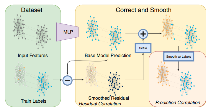
Simple base predictor

Here, a simple shallow MLP was used with softmax at the last layer and cross-entropy, as the loss function. This was trained on the training set. The validation set was used to tune hyperparameters such as learning rates, and the hidden layer dimensions. Finally, we obtain a matrix .

Correcting for error in base predictions with residual propagation

The key idea is that errors in base prediction to be possitively correlated along edges in the graph. In other words, an error at node increases the chances of a similar error at neighboring nodes of . For this, we first define an error matrix , where the error in residual on training data and zero everywhere else. We then smooth the error using label spreading technique optimizing an objective of two terms:

• First term encourages smoothness of error estimation over the graph
• The second terms keeps the solution close to the initial guess of the error.

After performing this step, we obtain the optimal . Adding this to gives us the corrected predictions. However, the optimal error might not be of the right scale, hence, we need to scale the residuals.

• Autoscale: Intuitively, the scale of size in errors in optimal to be approximately the size of errors in .
• Scaled Fixed Diffusion: Alternatively, we can use a diffusion which keeps the known erros at training nodes fixed. Intuitively, this fixes error values where we know the error (on labeled nodes ) while other nodes keep averaging over the values of their neighbors until convergence.

Smoothing final predictions with prediction correlation

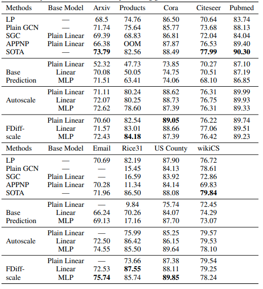
At this point, we have a score vector , obtained from collecting the base predictor with a model for the correlated error . To make a final prediction, we further smooth the corrected predictions. The motivation is that the adjacent nodes in the graph are likely to have similar labels, which is expected given homophily or assortative properties of a network. Thus, we can encourage smoothness over the distribution over labels by another label propagation. The performance of the model on the datasets is shown in the figure below.

Performance of the C&S model on different datasets.