An overview of the chapter “Numerical Computation” from the famous book “Deep Learning” written by Ian Goodfellow, Yoshua Bengio and Aaron Courville. The authors create a brief introduction of the important concepts from numerical computation that help guide machine learning. All images and tables in this post are from their book.

Introduction

Machine Learning algorithms usually require a very high amount of numerical computation: usually referring to algorithms that solve mathematical problems by methods that update estimates of the solution via an iterative process, rather than analytically deriving a formula providing a symbolic expression for the correct solution. Common operations include optimization and solving linear equations.

Overflow and Underflow

The fundamental difficulty in performing continuous math on a computer is that we need to represent infinitely many real numbers with a finite number of bit patterns. This means that for almost all real numbers, we incur some approximation error when we represent the number in the computer. In many cases, it would just be rounding error, but could cause problems when compunded across many operations.

• One form of rounding error is Underflow. Underflow occurs when numbers near zero are rounded to zero. Many functions behave qualitatively differently when their argument is zero rather than a small positive number. For instance, division by zero, or taking logarithm of zero.
• Another highly damaging form of numerical error is Overflow. Overflow occurs when very large numbers are rounded to or .

Poor Conditioning

Conditioning refers to how rapidly a function changes with respect to small changes in its inputs. Functions that change rapidly when their inputs are perturbed slightly can be problematic for scientific computation because rounding errors in the inputs can result in large changes in the output. Suppose where has an eigenvalue decomposition, its condition number is:

This is the ratio of the magnitude of the largest and smallest eigenvalue. When this number is large, matrix inversion is particularly sensitive to error in the input.

This sensitivity is an intrinsic property of the matrix itself, not the result of rounding error during matrix inversion. Poorly conditioned matrices amplify pre-existing errors when we multiply by the true matrix inverse.

Gradient-Based Optimization

Optimization refers to the task of either minimizing or maximizing some function by altering .The function we want to minimize or maximize is called the objective function or criterion. When we are minimizing it, we may also call it loss function, cost function or error function.

We denote the value that minimizes or maximizes a function with a superscript . For example, we might say .

An illustration of how the gradient descent algorithm uses the derivatives of a function can be used to follow the function downhill to a minimum.

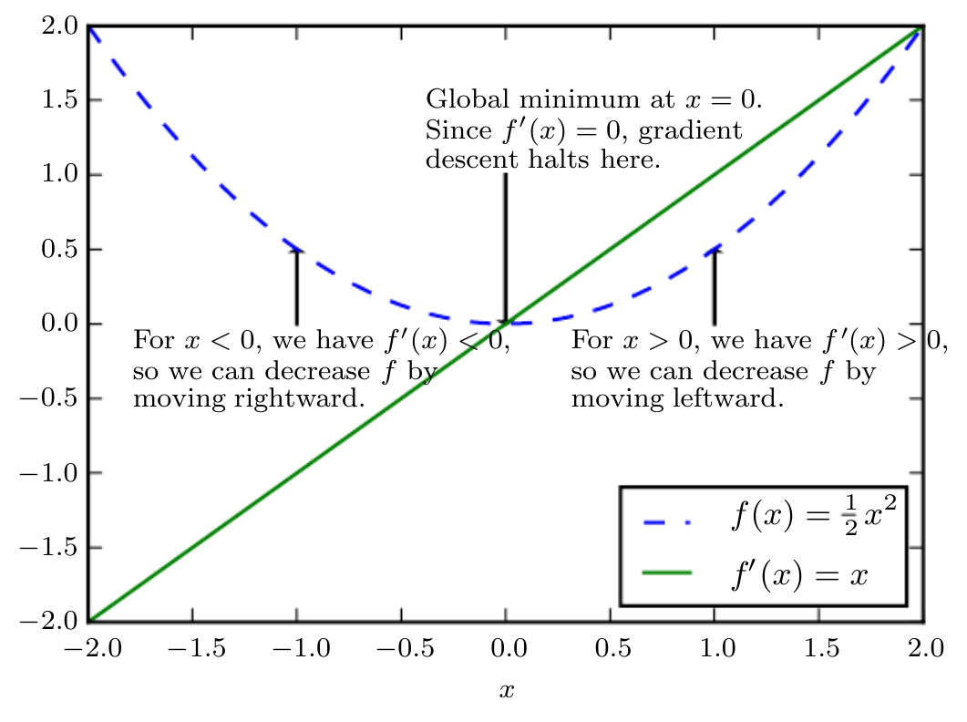
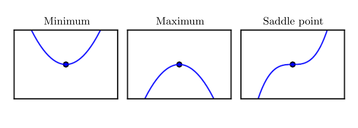
When , the derivative provides no information about which direction to move. Points where are known as critical points or stationary points. A local minima is a point where is lower than at all neighboring points, so it is no longer possible to decrease by making infinitesimal steps. A local maxima is a point where is higher than all neighboring points, so it is not possible to increase by making infinitesimal steps. Some critical points are neither mina or maxima, and are known as saddle points.

Examples of each of the three types of critical points in 1-D.

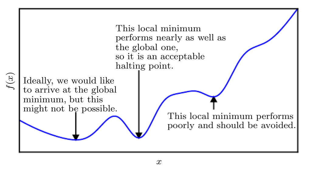
A point that obtains the absolute lowest value of is a global minimum. In the context of deep learning, we optimize functions that may have many local minima that are optimal, and many saddle points surrounded by very flat regions. All this makes optimization very difficult especially when the input to the function is multidimensional. We therefore settle for finding a value of that is very low but not necessarily the global minima in any formal sense.

For functions with multiple inputs, we must make use of the concept of partial derivatives. The partial derivative measures how changes as only the variable increases at point . The gradient generalizes the notion of derivative to the case where the derivative is with respect to a vector: The gradient of is the vector containing all of the partial derivatives, denoted . In multiple dimensions, critical points are points where every element of the gradient is equal to zero.

To minimize , we would like to find the direction in which decreases the fastest. We can do this using the directional derivative as follows:

where is the angle between and the gradient. The gradient points directly uphill, and the negative gradient points directly downhill. We can decrease by moving in the direction of the negative gradient. This is known as the method of steepest descent or gradient descent.

Gradient descent proposes a new point - where is the learning rate. Finding the right hyperparameter for the learning rate is quite important. To achieve this, it is quite common to perform a line search where we evaluate for several values of . Although, gradient descent is limited to optimization in continuous spaces, the general concept of repeatedly making a small move towards better configurations can be generalized to discrete spaces. Ascending an objective function of discrete parameters is called hill climbing.

Note that optimization algorithms may fail to find a global minimum when there are multiple local minima or plateaus present. In the context of deep learning, we generally accept such solutions even though they are not truly minimal, so long as they correspond to significantly low values of the cost function as shown below.

Jacobian and Hessian Matrices

Sometimes, we need to find all of the partial derivatives of a function whose input and output are both vectors. The matrix containing all such partial derivatives is known as the Jacobian matrix. Specifically, we would have a function , then the Jacobian matrix of is defined such that .

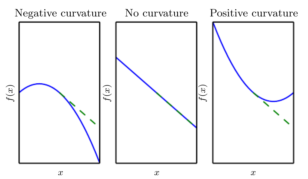
We are sometimes also interested in the second order derivative. The second derivative tells us how the first derivative will change as we vary the input. This is important because it tells us whether a gradient step will cause as much of an improvement as we would expect based on the gradient alone. We can think of the second derivative as measuring the curvature, as shown in the figure below.

When our function has multiple input dimensions, there are many second derivatives. These derivatives can be collected together into a matrix called the Hessian matrix. The Hessian matrix is defined such that:

Anywhere the second partial derivatives are continuous, the differential operators are commutative, i.e. their orders can be swapped:

This implies that , and the Hessian matrix is symmetric in nature. Since the Hessian matrix is real and symmetric everywhere in the context of deep learning, we can decompose it into a set of real eigenvalues and an orthogonal basis of eigenvectors. The second derivative is a specific direction represented by a unit vector is given by . When is an eigenvector of , the second derivative in that direction is given by the corresponding eigenvalue. For other directions of , the directional second derivative is a weighted average of all of the eigenvalues, with weights between 0 and 1, and eigenvectors that have smaller angle with receiving more weight.

The second derivative tells us how well we can expect the gradient descent to perform. We can make a second-order Taylor-series approximation to the function around the current point :

where is the gradient and is the Hessian at . If we use a learning rate of , then the new point will have the value:

There are three terms here:

• the original value of the function
• The expected improvement due to the slope of the function
• The correction we must apply to account for the curvature of the function.

When the last term is too large, the gradient descent step can actually move uphill. When the third term is zero or negative, the approximation predicts that increasing the learning rate forever will decrease forever. However, in practice, the Taylor series is unlikely to remain accurate for large , so one must resort to more heuristic choices of in this case. However, when the last term is positive, solving for the optimal step size that decreases the Taylor series approximation of the function the most yields:

Tests for finding nature of critical points

Furthermore, the second derivative can be used to determine whether a critical point is a local maxima, a local minima or saddle point. Note that on a critical point, . So,

• If , then it is local minima.
• If , then it is local maxima.
• If , then the test is inconclusive. The point could be a saddle point, or a part of a flat region.

In multiple dimensions, we need to examine all of the second derivatives of the function. At a critical point, where , we can examine the eigenvalues of the Hessian to determine whether the critical point is a local maxima, local minima or saddle point.

• When the Hessian is positive definite (all its eigenvectors are positive), the point is a local minima.
• When the Hessian is negative definite (all its eigenvectors are negative), the point is a local maxima.
• When atleast one positive and negative eigenvector exists of a given Hessian, there is a possibility of a saddle point, but the test remains inconclusive.

Limitations of Gradient Descent, and Proposed Solution

In multiple dimensions, there is a different second derivative for each direction at a single point. The condition number of the Hessian at this point measures how much the second derivatives differ from each other. When the Hessian has a poor condition number, gradient descent performs poorly. This is because in one direction, the derivative increases rapidly, while in another direction, it increases slowly. Gradient descent is unaware of this change in derivative so it does not know that it needs to explore preferentially in the direction where the derivative remains negative for longer.

However, this issue can be resolved by using information from the Hessian matrix to guide the search. The simplest method for doing so is known as Newton’s method. Newton’s method is based on using a second-order Taylor series expansion to approximate near some point . We update such that:

• When is a positive definite quadratic equation, Newton’s method jumps directly to the minimum of the function.
• When is not truly quadratic but can be locally approximated as a postive definite quadratic, applying Newton’s method multiple times helps reach the critical point much faster than gradient descent.

This is a very useful property near a local minima, but can become highly harmful when near a saddle point. Newton’s method is only appropriate when the nearby critical point is a minimum, whereas gradient descent is not attracted to saddle points unless gradient points towards them.

Optimization algorithms that use only the gradient such as gradient descent are called first-order optimization algorithms. Optimization algorithms that also use the Hessian matrix, such as Newton’s method are called second-order optimization algorithms.

Lipschitz continuous functions

In the context of deep learning, we sometimes gain some guarantees by restricting ourselves to functions that are either Lipschitz continuous or have Lipschitz continuous derivatives. A Lipschitz continuous function is a function whose rate of change is bounded by a Lipschitz constant :

This property is useful because it allows us to quantify our assumption that a small change in the input made by an algorithm such as gradient descent will have a small change in the output. Lipschitz continuity is also a fairly weak constraint, and many optimization problems in deep learning can be made Lipschitz continuous with relatively minor modifications.

Convex Optimization

Perhaps the most successful field of specialized optimization is convex optimization. Convex optimization algorithms are able to provide many more guarantees by making stronger restrictions. Convex optimization algorithms are applicable only to convex functions - functions for which the Hessian is positive semidefinite everywhere. Such functions are well-behaved because they lack saddle points and all of their local minima are necessarily global minima. However, most problems in deep learning are difficult to express in terms of convex optimization.

Constrained Optimization

Sometimes we wish not only to maximize or minimize a function over all possible values of . Instead, we may mish to find the maximal or minimal value of for values of in some set . This is known as constrained optimization. Points that lie within the set are called feasible points in constrained optimization terminology. We often wish to find a solution that is small in some sense. A common approach in such situations is to impose a norm constraint, such as . There are few approaches to help solve this problem:

Approach #1:

A simple approach is to simply modify gradient descent taking the constraint into account. If we use a small constant step size , we can make gradient descent steps, then project the result back into . If we use a line search, we can only search over step sizes that yield new points that are feasible, or we can project each point on the line back into the constraint region. When possible, this method can be made more efficient by projecting the gradient into the tangent space of the feasible region before taking the step.

Approach #2:

A more sophisticated approach is to design a different, unconstrained optimization problem whose solutions can be converted into a solution to the original constrained optimization problem. For example, if we want to minimize for with constrained to have exactly unit norm, we can instead minimize with respect to , then return as the solution to the original problem. This approach is less generic and requires creativity for each case we encounter.

Approach #3:

The Karush-Kuhn-Tucker (KKT) approach provides a more general solution to constrained optimization. This approach introduces the lagrange optimization procedure. Suppose we want a description of in terms of equality constraints and inequality constraints . To optimize this equation, we introduce new variables and for each constraint. These variables are called the KKT multipliers. The generalized Lagrangian is then defined as:

With this simple conversion, we can solve the constrained optimization problem similar to our unconstrained optimization problem. A simple set of properties describe the optimal points of constrained optimization problems. These properties are called the Karush-Kuhn-Tucker (KKT) conditions. They are necessary conditions, but not always sufficient conditions for a point to be optimal. The conditions are:

• The gradient of the generalized Lagrangian is zero.
• All constraints on both . and the KKT multipliers are satisfied.
• The inequality constraints exhibit “complementary slackness”, i.e. .