Probability and Information Theory

An overview of the chapter “Probability and Information Theory” from the famous book “Deep Learning” written by Ian Goodfellow, Yoshua Bengio and Aaron Courville. The authors create a brief introduction of the important concepts of probability and information theory that help guide machine learning. All images and tables in this post are from their book.

Introduction

Probability can be seen as the extension of logic to deal with unceratinty. Probability can be viewed in two ways:

Bayesian Probability: This indicates the certainty or the degree of belief that the event occurs. A degree of belief of 1 indicates absolute certainty of the event. This probability is qualitative in nature.
Frequentist Probability: This indicates the rate at which the event occurs. This probability is quantitative in nature.

Random Variables

A random variable is a variable that can take on different values randomly. These may be discrete or continuous. A discrete random variable is one that has a finity or countably infinite number of states. These nese states are not necessarily integers, and can also just be named states that are not considered to have any numberical value. A continuous random value is associated with a real value.

Probability Distributions

A probability distribtuion is a description of how likely a random variable or set of random variables is to take on each of its possible states. THe way we describe probability distributions depend on whether the variables are discrete or continuous.

Discrete Variables and Probability Mass Functions

A probability over discrete variables may be described using a probability mass function. The probability of the event $x$ taking place is $P(x)$ . If there are more than one variable, we define a joint probability distribution as $P(x,y)$ . To be a probability mass function on a random variable $x$ , a function $P$ must satisfy the following properties:

The domain of $P$ must be the set of all possible states of $x$ .
$\forall x, 0\leq P(x)\leq 1$
$\sum_{x}P(x) =1$

For example, consider uniform distribution where all the states are equally likely. Suppose there are $k$ states, the probability mass function is:

$P(x=x_i)=\frac{1}{k}$

Continuous Variables and Probability Density Functions

While working with continuous random variables, we describe probability distributions using a probability density function rather than a prabability mass function. To be a probability density function, a function $p$ must satisfy the following properties:

The domain of $p$ must be the set of all possible states of $x$ .
$\forall x, p(x)\geq 0$
$\int p(x)dx = 1$

The probability of event between $a$ and $b$ , can be obtained by computing $\int_{a}^{b} p(x)dx$ . Also the probability of an event $a$ occuring is 0, since $\int_{a}^{a} p(x)dx = 0$ .

Marginal Probability

The probability over a subset is known as the marginal probability distribution. For discrete variables, $\forall x, P(x) = \sum _y P(x,y)$ . For continuous variables, $\forall x, p(x) = \int p(x,y)dy$ .

Conditional Probability

Conditional probability is the probability of some event, given that some other event has happened.

$P(y|x) = \frac{P(x,y)}{P(x)}$

The conditional probability is only defined when $P(x)>0$ , we cannot compute the conditional probability conditioned on an event that never happens. It is important not to confuse conditional probability with computing what would happen if some action were undertaken. Computing the conequences of an action is called making an intervention queries. Intervention queries are the domain of causal modeling.

The Chain Rule of Conditional Probabilities

Any joint probability distribution over many random variables may be decomposed into conditional distributions over only one variable:

$P(a,b,c)=P(a|b,c)P(b,c) = P(a|b,c)P(b|c)P(c)$

Independence and Conditional Independence

Two variables $x$ and $y$ are independent if their probability distribution can be expressed as a product of two factors, one involving only $x$ and one involving only $y$ :

$P(x,y) = P(x)P(y) \Leftrightarrow P(x|y) = P(x)$

Two random variables $x$ and $y$ are conditionally independent given a random variable $z$ if the conditional probability distribution over $x$ and $y$ factorizes in this way for every value of $z$ :

$P(x,y|z)=P(x|z)P(y|z) \Leftrightarrow P(x|y,z) = P(x|z)$

We can denote the independence with compact notation: $x\perp y$ means that $x$ and $y$ are independent, while $x\perp y |z$ means that $x$ and $y$ are conditionally independent given $z$ .

Expectation, Variance and Covariance

Expectation

The expectation or expected value of some function $f(x)$ with respect to a probability distribution $P(x)$ is the average or mean value that $f$ takes on when $x$ is drawn from $P$ . For discrete variables:

$\mathbb{E}_{x\sim P}[f(x)] = \sum_x P(x)f(x)$

For continuous variables:

$\mathbb{E}_{x\sim p}[f(x)] = \int_x p(x)f(x)dx$

Moreover, expectations are linear, for example,

$\mathbb{E}_{x}[\alpha f(x) + \beta g(x)] = \alpha \mathbb{E}_{x}[f(x)] + \beta \mathbb{E}_{x}[g(x)]$

when $\alpha$ and $\beta$ are not dependent on $x$ .

Variance

The variance gives a measure of how much the values of a function of a random variable $x$ vary as we sample different values of $x$ from its probability distribution:

$Var(f(x)) = \mathbb{E}[(f(x)-\mathbb{E}[f(x)])^2]$

When the variance is low, the values of $f(x)$ cluster near their expected value. The square root of the variance is known as the standard deviation.

Covariance

The covariance gives some sense of how much to values are linearly related to each other, as wlel as the scale of these variables:

$Cov(f(x),g(y)) = \mathbb{E}[(f(x)-\mathbb{E}[f(x)])(g(y)-\mathbb{E}[g(y)])]$

High absolute values of the covariance mean that the values change very much and are both far from their respective means at the same time. If the sign of the covariance is positive, then both variables tend to take on relatively high values simultaneously. If the sign of the covariance is negative, then one variable tends to take on a relatively high value at the times that the other takes on a relatively low value and vice versa. Other measures such as correlation normalize the contribution of each variable in order to measure only how much the variables are related, rather than also veing affected by the scale of the seperate variables. The notions of covariance and dependence are related but still distinct. If the covariance is zero, the two variables are linearly dependent. However, there could also be cases where the variables show non-linear dependency and covariance is not zero. However, there cannot be dependency if the covariance is not zero. The covariance matrix of a random vector $x \in \mathbb{R}^n$ is an $n*n$ matrix, such that

$Cov(x)_{i,j} = \left\{\begin{matrix} Cov(x_i,x_j) & ,i\neq j\\ Var(x_i) & ,i=j \end{matrix}\right.$

Common Probability Distribution

Bernoulli Distribution

The bernoulli distribution is a distribution over a single binary random variable.

$P(x=1) = \Phi$
$P(x=0) = 1-\Phi$
$P(x) = \Phi^x(1-\Phi)^{1-x}$
$E_x[x] = \Phi$
$Var_x(x) = \Phi(1-\Phi)$

Multinomial Distribution

THe mulitnomial distribution is a distribution over a single discrete variable with $k$ different states, where $k$ is finite. Multinoulli distributions are often used to refer to distributions over categories of objects, so we do not usually assume that state 1 has numerical value 1, etc. For this reason, we do not usually need to compute the expectation or variance of multinoulli-distributed random variables.

$P(x) = \Phi^x(1-\Phi)^{n-x}$

Gaussian Distribution

The most commonly used distribution over real numbers is the normal distribution, also known as the gaussian distribution.

$N(x;\mu ,\sigma ^2) = \frac{1}{\sqrt{2\Pi}\sigma}e^{-\frac{(x-\mu)^2}{2\sigma^2}}$
$E_x[x] = \mu$
$Var_x(x) = \sigma^2$

When we need to frequently evaluate the PDF with different parameter values, a more efficient way parametrizing the distribution is to use a parameter $\beta$ to control the precision or inverse variance of the distribution, $\beta = \sigma^{-2}$

In the absence of prior knowledge about what form a distribution over the real numbers should take, the normal distribution is a good default choice for two major reasons:

Many distributions we wish to model are truly close to being normal distributions. The central limit theorem shows that the sum of many independent random variables is approximately normally distributed. This means that in practice, many complicated systems can be modeled successfully as normally distributed noise, even if the system can be decomposed into parts with more structured behavior.
Out of all possible probability distributions with the same variance, the normal distribution encodes the maximum amount of uncertainty over the real numbers. We can thus think of the normal distribution as being the one that inserts the least amount of prior knowledge into a model. The normal distribution generalizes to $\mathbb{R}^{n}$ , in which case it is known as the multivariate normal distribution. It may be parametrized with a positive definite symmetric matrix $\sum$ :

$N(x;\mu ,\sum ) = \frac{1}{(2\Pi)^{n/2}\left | \sum \right |^{0.5}} e^{-\frac{1}{2}(x-\mu)^T\sum ^{-1}(x-\mu)}$

where $\mu$ is mean, and $\sum$ is covariance matrix. We often fix the covariance matrix to be a diagonal matrix. An even simpler version is the isotropic Gaussian distribution, whose covariance matrix is a scalar times the identity matrix.

Exponential and Laplace Distributions

In the context of deep learning, we often want to have a probability distribution with a sharp point at $x=0$ . To accomplish this, we can use the exponential distribution:

$P(x;\lambda) = \lambda e^{-\lambda x}$

A closely related probability distribution that allows us to place a sharp peak of probability mass at an arbitrary point $\mu$ is the Laplace distribution:

$Laplace(x;\mu,,\gamma ) = \frac{1}{2\gamma }e^{-\frac{\left | x-\mu \right |}{\gamma }}$

The Dirac Distribution and Empirical Distribution

In some cases, we wish to specify that all of the mass in a probability mass in a probability distribution clusters around a single point. This can be accomplished by defining a PDF using the Dirac delta function, $\delta (x)$ . The Dirac delta function is defined such that is is zero-valued everywhere except 0, yet integrates to 1. Dirac function is not an ordinary fucntion and falls under the category of generalized function.

A common use of the Dirac delta distribution is as a component of an empirical distribution,

$\hat{p}(x) = \frac{1}{m}\sum _{i=1}^{m}\delta (x-x^{(i)})$

which puts a probability mass $\frac{1}{m}$ on each of the $m$ points $x^{(1)},...,x^{(m)}$ forming a given dataset or collection of samples.

Mixtures of Distributions

A mixture distribution is made up of several component distributions. On each trial, the choice of whihc component distribution generates the sample is determined by sampling a component identity from a multinomial distribution:

$P(x) = \sum _i P(c=i)P(x|c=i)$

where $P(c)$ is the multinomial distribution over component identities.

A latent variable is a random variable that we cannot observe directly. The component identity variable $c$ of the mixture model provides an example. Latent variables may be related to $x$ through the joint distribution, in this case, $P(x,c) = P(x|c)P(c)$ . The distribution $P(c)$ over the latent variable and the distribution $P(x|c)$ relating the latent variables to the visible variables determines the shape of the distribution $P(x)$ even though it is possible to describe $P(x)$ without reference to the latent variable.

A very powerful and common type of mixture model is the Gaussian mixture model, in which the components $P(x|c=i)$ are Gaussians. We would also need to specify the prior probability $\alpha _i = P(c=i)$ given to each component $i$ . The word “prior” is used since it expresses the model’s beliefs about $c$ before it observes $x$ . By comparison, $P(c|x)$ is a posterior probability, because it is computed after observation of $x$ . A Gaussian mixture model is a universal approximator of densities, in the sense that any smooth density can be approximated with any specific, non-zero amount of error by a Gaussian mixture model with enough components.

Useful Properties of Common Functions

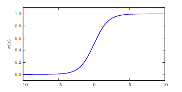
Logistic Sigmoid:

$\sigma (x) = \frac{1}{1+\exp(-x)}$

The sigmoid function saturates when its argument is very positive or very negative, meaning that the function becomes very flat and insensitive to small changes in its input.

The logistic sigmoid function.

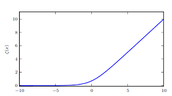
Softplus function:

$\zeta (x) = \log(1+\exp(x))$

The name of softplus function comes from the fact that it is a smoothed or “softened” version of ReLU.

The softplus function.

The following properties are all useful enough to memorize:

$\sigma (x) = \frac{\exp(x)}{\exp(x)+\exp(0)}$
$\frac{\mathrm{d}}{\mathrm{d} x} \sigma(x) = \sigma(x)(1-\sigma(x))$
$1-\sigma(x) = \sigma(-x)$
$\frac{\mathrm{d} }{\mathrm{d} x}\zeta (x) = \sigma(x)$
$\sigma^{-1}(x) = \log(\frac{x}{1-x})$
$\zeta ^{-1}(x) = \log(\exp(x)-1)$
$\zeta(x) = \int_{-\infty}^{x} \sigma(y)dy$
$\zeta(x) - \zeta(-x) = x$

The function $\sigma^{-1}(x)$ is called the logit in statistics.

Bayes’ Rule

$P(x|y) = \frac{P(x)P(y|x)}{P(y)}$

Although $P(y)$ appears to be in the formula, it is usually feasible to compute $P(y) = \sum _x P(y|x)P(x)$ so we do not need to begin with knowledge of $P(y)$ .

Technical Details of Continuous Variables

Measure zero is a convept which is used to define a very small set of points. Another useful term is almost everywhere where a property holds throughout all of space except for on a set of measure zero. Another technical detail of continuous variables relates to handling continuous random variables that are deterministic functions of one another. Suppose we have two random variables, $x$ and $y$ , such that $y = g(x)$ . One might expect that $p_y(y) = p_x(g^{-1}(y))$ which is not the case.

For higher dimensions, the derivative generalizes to the determinant of the Jacobian matrix, the matrix with $J_{i,j}= \frac{\partial x_i}{\partial y_j}$ .

Information Theory

The basic intuition behind information theory is that learning that an unlikely event has ovvured is more informative than learning that a likely event has occured. A common function used is the self-information of an event $x$ to be

$I(x) = -\log P(x)$

Here, we mean to use natural logarithm, with base $e$ and wriiten in units of nats. Others use a base-2 logarithms and units called bits or shannons. However, the self-information deals with only a single outcome.

We can quantify the amount of uncerainty in an entire probability distribution using the Shannon entropy:

$H(P) = \mathbb{E}_{x\sim P}[I(x)] = -\mathbb{E}_{x\sim P}[\log P(x)]$

When x is continuous, the Shannon entropy is known as the differential entropy. If we have two seperate probability distributions $P(x)$ and $Q(x)$ over the same random variable $x$ , we can measure how different these two distributions are using the Kullback-Leibler (KL) divergence:

$D_KL(P||Q) = \mathbb{E}_{x\sim P}\begin{bmatrix} \log \frac{P(x)}{Q(x)} \end{bmatrix}$

In the case of discrete variables, it is the extra amount of information needed to send a message containing symbols drawn from probability distribution $P$ , when we use a code that was designed to minimize the length of messages drawn from probability distribution $Q$ .

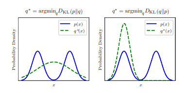
The KL divergence has many useful properties, most notably that it is nonnegative.The KL divergence is 0 if and only if $P$ and $Q$ are the same distribution in the case of discrete variables, or equal “almost everywhere” in the case of continuous variables. Because the KL divergence is non-negative and measures the difference between two distributions, it is often conceptualized as measuring some sort of distance between these distributions. However, it is not a true distance measure because it is not symmetric: $D_{KL}(P||Q) \neq D_{KL}(Q||P)$ for some $P$ and $Q$ . This asymmetry means that there are important consequences to the choice of whether to use $D_{KL}(P||Q)$ or $D_{KL}(Q||P)$ .

KL divergence is assymetric.

A quantity that is closely related to the KL divergence is the cross-entropy $H(P,Q) = H(P) + D_{KL}(P||Q)$

Structured Probabilistic Models

Machine learning algorithms often involve probability distributions over a very large number of random variables. Using a single function to describe the entire joint probability distribution can be very inefficient (both computationally and statistically). Instead of using a single function to represent a probability distribution into many factors that we multiply together. These factorizations can be describes using graphs and call them structured probabilistic model or graphical model. There are two main kinds of structured probabilistic models: directed and undirected

Directed Models

Graphs with directed edges, and they represent factorizations into conditional probability distributions.

Directed model.

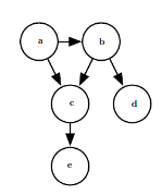
Here, $p(a,b,c,d,e) = p(a)p(b|a)p(c|a,b)p(d|b)p(e|c)$

Undirected Models

Graphs with undirected edges, and represent factorizations into a set of functions. Usually, these functions are not probability distributions of any kind. Any set of nodes that are all connected to each other in $G$ is called a clique. Each clique $C^{(i)}$ in an undirected model is associated with a factor $\Phi ^{(i)}(C^{(i)})$ . The output of each factor must be non-negative, but there is no constraint that the factor must sum or integrate to 1 like a probability distribution.

Undirected model.

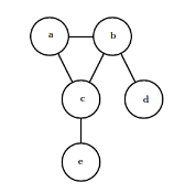
Here, $p(a,b,c,d,e) = \frac{1}{Z}\Phi ^{(1)}(a,b,c)\Phi ^{(2)}(b,d)\Phi ^{(3)}(c,e)$ .

Written on January 11, 2021