An overview of the paper “Invariance Principle Meets Information Bottleneck for Out-of-Distribution Generalization”. In this paper, the authors propose an approach called the IB-IRM approach that would fare well even in OOD distribution cases. All images and tables in this post are from their paper.

Introduction

The success of deep learning has been truly remarkable. However, recent years have witnessed an explosion of examples showing deep learning models are prone to exploiting shortcuts (spurious features) which fail to generalize out-of-distribution (OOD). The paper motivates this problem with the example of the problem of cow-camel-classification. For instance, a convolutional neural network trained to classify camels from cows; however, it was found that the model relied on the background color (e.g., green pastures for cows) and not on the properties of the animals (e.g., shape). This is a classic example of causation is not the same as correlation.

Background

Intervention is defined as the model distribution shifts (images from different locations). This definition is consistent with the theory from causal learning. The cause is defined as a subset of features invariant across all interventions. The training set is denoted by , and the set of all examples including training is denoted by . The network is defined as where the error is defined as where . The idea of this loss is to minimize the maximum loss obtained by OOD.

Structural Equation Model (SEM)

In such cases, the input sample is defined as , where is the input sample. are the latent invariant features and are the latent spurious features. Furthermore, is the function that maps these latent features to the actual input to the model. Furthermore, this model also assumes that the output feature , where the output feature is solely dependent on the invariant features with some added gaussian noise. Under this setting, we also assume the functions and to be constant, and is trained to minimize OOD.

Invariant Risk Minimization (IRM)

Before we understand IRM, it is important to discuss what invariant predictors are. Suppose a network is defined as , where is the classifier and is the reprentator. If the representator is fixed, and we allow changes to the classifier depending on the environment, and the classifer converges to the same weights everytime, we call the model an invariant predictor.

In IRM, the goal is , where is the invariant predictor. If the condition that is an invariant predictor is dropped, we reach the Empirical Risk Minimization setting.

If , are linear, IRM would be optimal, but ERM would fail. However, it is possible for both ERM and IRM to fail in cases of linear classification as shown in the example below:

Failures of ERM and IRM in linear classification

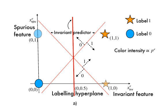
As shown in the figure, If latent invariant features in the training environments are separable, then there are multiple equally good candidates that could have generated the data, and the algorithm cannot distinguish between these. The models that use the spurious features for their prediction are bad classifiers, and would be easy to provide a counter-example in OOD setting where the model fails.

2-D fully informative invariant features (FIIF)

In this setting, the invariant features are assumed to have all the information for the models. The inputs are defined as and the outputs are defined as where is the bernoulli distribution. The above setting comes with a few assumptions:

• Bounded invariant features: is a bounded set.
• Bounded spurious features: is a bounded set.
• Invariant feature support overlap:
• Spurious feature support overlap:

Note that, the last two assumptions state that the support set of the invariant (spurious) features for unseen environments is the same as the union of the support over the training environments. However, support overlap does not imply that the distribution over the invariant features does not change. Furtherore, to measure how much the training support of invariant features is seperated by the labelling hyperplane , the authors define Inv-margin as . If the Inv-Margin is greater than 0, then the labelling hyperplane seperates the support set into two halves. 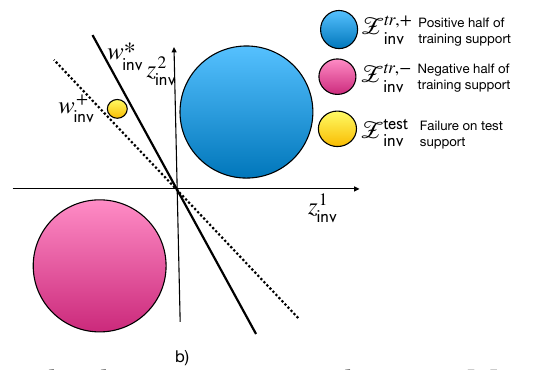The authors further show that if the support of latent invariant features are strivtly separated by the labelling hyperplane , then we can find another valid hyperplane that is equally likely to have generated the same data. There is no algorithm that distinguish between the two hyperplanes. As a result, if we use data from the region where the hyperplanes disagree (yellow region), then the algorithm fails.

Impossibility result

Thus, even if invariant support overlap is guaranteed, the model could still fail if the model relies on spurious changes. However, if spurious features are kept constant, then both ERM and IRM could potentially succeed.

Invariance + IB

The idea in this setting is to pick the classifer with minimum differential entropy. This would allow the model to keep as less information about the spurious features. The proposed approach is able to succeed in all the above cases where IRM or ERM fail. The authors propose a new loss in order to train in this setting, which involves the ERM loss, IRM V1 penalty and the variance penalty.