An overview of the topic “Meta-Learning: Learning to Learn Fast blog” and “Meta-Learning: Learning to Learn Fast ICML tutorial”. A good meta-learning model should be capable of well adapting or generalizing to new tasks and environments that have never been encountered during training time. This is why meta-learning is known as “learning to learn”. All images and tables in this post are from their respective paper. The idea here is to create algorithms when the following scenarios exist:

• Do not have a large dataset
• Want a general-purpose AI system in the real world. This would need to continuously adapt and learn on the job. Learning each thing from scratch wouldn’t cut it.
• When the data has a long tail, i.e., some classes or labels have very few examples when compared to other classes. In all three settings, the supervised learning paradigm is being broken. For us humans, we use previous experience to support our prediction. There are two views to view meta learning. Note that the two views below are not describing different algorithms, but could be different views of the same algorithm.

Mechanistic View

• Deep neural network model that can read in an entire dataset and make predictions for new datapoints.
• Training this network uses a meta-dataset which itself consists of many datasets, each for a different task.
• This view makes it easier to implement meta-learning algorithms

Probabilistic View

• Extract prior information from a set of tasks that allow efficient learning of new tasks
• Learning a new task uses this prior and (small) training set to infer most likely posterior parameters.
• This view makes it easier to understand meta learning algorithms.

Defining the Meta-Learning Model

The simple meta-training problem can be described as where, is the dataset we want to optimize for, and is the additional data we would like to use for this classification. However, if we do not want to use forever, we would need to boil down to another representation, say . This is the process of learning meta-parameters(). The meta-learning problem boils down to the equation . This allows us to classify the samples in using the following equation:

Applying argmax on both sides, we obtain the equation for adaptation: The complete picture of meta-learning involves learning of which is good for .

A simple view

A good meta-learning model should be trained over a variety of learning tasks and optimized for the best performance on a distribution of tasks, potentially unseen tasks. The optimal model parameters are:

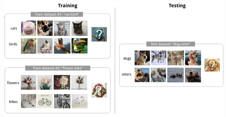
This is very similar to a normal learning task, but one dataset is considered as one data sample. Few-shot classification is an instantiation of meta-learning in the field of supervised learning. The dataset is often divided into two parts, a support set for learning and a prediction set for training or testing, . Often we consider a K-shot N-class classification task: the support set contains labelled examples for each of classes.

An example for 2-way 4-shot image classification.

Training in the same way as testing

A dataset contains pairs of feature vectors and labels, where each labels belong to a known label set . Our classifer , like any other classifier with parameter outputs a probability of a data point belonging to the class given the feature vector , . The optimal parameters maximize the probability of true labels across multiple training batches.

In few-shot classification, the goal is to reduce the prediction error on data samples with unknown labels given a small support set for “fast learning” (similar to fine-tuning). To make the training process mimic what happens during inference, we would like to “fake” datasets with a subset of labels to avoid exposing all lables and modify the optimization procedure such as:

• Sample a subset of labels .
• Sample a support set and a training batch . Both of them only contain data points with labels belonging to the sampled label set .
• The support set is part of the model input
• The final optimization uses the mini-batch to compute the loss and update the model parameters ().

Note, that the new optimal parameters is computed using:

Learning as Meta-Learner

A popular view of meta-learning decomposes the model update into two stages:

• A classifier is the learner model trained for operating a given task.
• In the meantime, a optimizer learns how to update the learner model’s parameters via the support set .

There are four common approaches to meta-learning: metric-based, model-based and optimization-based, and bayesian approach.

Metric-Based

The core idea in metric based meta-learning is similar to nearest neighbors algorithm and kernel density estimation. The predicted probability over a set of known labels is a weighted sum of labels of support set samples. The weight is generated by a kernel function , measuring the similarity between two data samples. These methods are also called non-parametric methods.

All the models introduced introduced below learn embedding vectors of input data explicitly and use them to design proper kernel functions.

Convolutional Siamese Neural Network

The siamese neural network is composed of two twin networks and their outputs are jointly trained on top with a function to learn the relationship between pairs of input data samples. The twin networks are identical, sharing the same weights and network parameters. In other words, both refer to the same embedding network that learns an efficient embedding to reveal relationship between pairs of data points. Koch et al. proposed a method to use the siamese neural network to do one-shot image classification. First, the siamese network is trained for a verification task for twlling whether two input images are in the same class. It outputs the probability of two images belonging to the same class. Then, during test time, the siamese network processes all the image pairs between a test image and every image in the support set. The final prediction is the class of the support image with the highest probability. Here, meta-training would be a 2 way classification problem, and the meta-testing would be a N-way classification problem.

The architecute of convolutional siamese neural network for few-shot image classificaation.

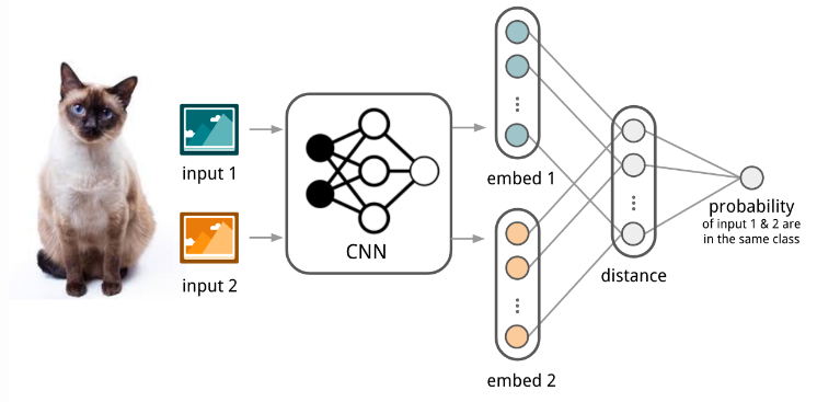
• First, convolutional siamese network learns to encode two images into feature vectors via a embedding function which contains a couple of convolutional layers.
• The L1-distance between two embeddings is .
• The distance is converted into a probability by a linear feedforward layer and sigmoid. It is the probability of whether two images are drawn from the same class.
• Intuitively the loss is cross entropy because the label is binary.

The assumption is that the learned embedding can be generalized to be useful for measuring the distance between images of unknown categories. This is the same assumption behind transfer learning via the adoption of a pre-trained model; for example, the convolutional features learned in the model pre-trained with ImageNet are expected to help other image tasks. However, the benefit of a pre-trained model decreases when the new task diverges from the original task that the model was trained on.

Matching Networks

The task of matching networks proposed by Vinyals et al. is to learn to classify for any given support set . This classifier defines a probability distribution over output labels given a test example . Similar to other metric-based models, the classifier output is defined as a sum of labels of support samples weighted by attention kernel - which should be proportional to the similarity between and .

The architecute of Matching Networks.

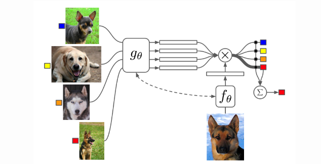
The attention kernel depends on two embedding functions, and , for encoding the test sample and the support set samples respectively. The attention weight between two data points is the cosine similarity between their embedding vectors, normalized by softmax:

In the Simple embedding version, an embedding function is a neural network with a single data sample as input. Potentially, we can set .

However, the embedding vectors are critical inputs for building a good classifier and taking a single point might not be efficient. Hence, we create full context embeddings. The matching network model further proposed to enhance the embedding functions by taking as input the whole support set in addition to the original input, so that the learned embedding can be adjusted based on the relationship with other support samples.

• uses a bidirectional LSTM to encode in the context of the entire support set .
• encodes the test sample via an LSTM with read attention over the support set . First the test sample goes through a simple neural network to extract basic features. Then an LSTM is trained with a read attention vector over the support set as part of the hidden state. This embedding method does help performance on a hard task (few-shot classification on mini Imagenet) but makes no difference on a simple task (Omniglot). However, if we have a N-shot problem where , then the model would compare the test sample with each image of each sample of every class. This challenge lead to the creation of an aggregation of class information, also called prototypical embedding which is used in the Prototypical networks, which are discussed later.

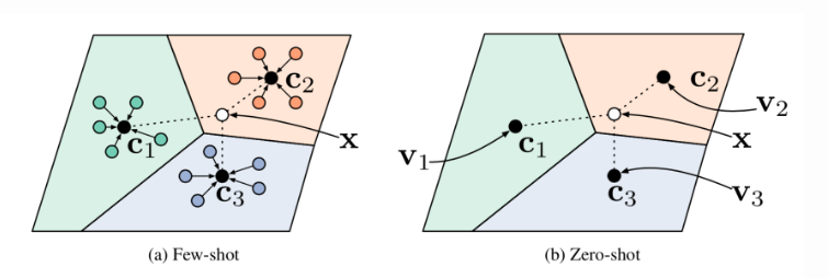
Prototypical Networks

Prototypical networks proposed by Snell et al. uses an embedding function to encode each input into a -dimensional feature vector. A prototype feature vector is define for every class as the mean vector of embedded support data samples in this class. The prediction is made by computing the softmax of distances between these prototypical mean embeddings and query set or test set.

Prototypical networks in the few-shot and zero-shot scenarios.

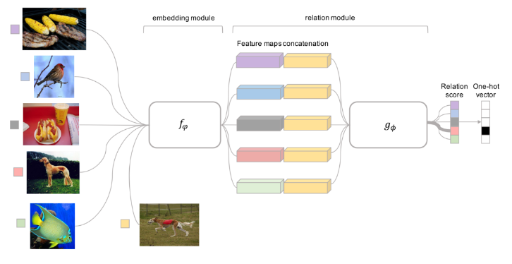
Relation Network

Relation Network was proposed by Sung et al., and is similar to the siamese network with a few differences:

• The relationship is not captured by a simple L1 distance in the feature space, but predicted by a CNN classifier . The relation score between a pair of inputs and , is where is concatenation.
• The objective function is MSE loss, vecause conceptually RN focuses more on predicting relation scores which is more like regression, rather than binary classification.

Relation Network architecture for a 5-way 1-shot problem with one query example.

This addresses the challenge faced by the previous methods, where we need to model more complex relationships between datapoints. In this method, we learn non-linear relation module on embeddings. Other solutions to the challenge include:

• Learning infinite mixture of prototypes, or
• Perform message passing on embeddings using GNN

Model-Based

Model-based met-learning models make no assumption on the form of . Rather, it depends on a model designed specifically for fast learning. This rapid parameter update can be achieved by its internal architecture or controlled by another meta-learner model.

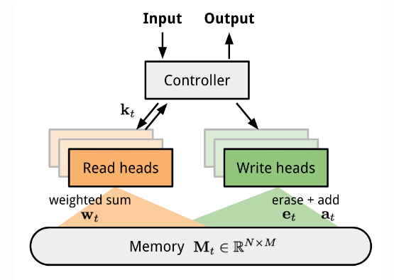
Memory-Augmented Neural Networks

A family of model architectures use external memory storage to facilitate the learning process of neural networks, including Neural Turing Machines and Memory Networks. With an explicit storage buffer, it is easier for the network to rapidly incorporating new information and not to forget in the future. Such a model is known as MANN. Because MANN is expected to encode new information fast and thus to adapt to new tasks after only a few samples, it fits well for meta-learning. Neural Turning Machines couples a controller neural network with external memory storage. The controller learns to read and write memory rows by soft attention, while the memory serves as a knowledge repository. The attention weights are generated by its addressing mechanism: content-based+location based.

The architecture of Neural Turning Machine.

To use MANN for meta-learning tasks, we need to train it in a way that memory can encode and capture information of new tasks fast and, in the meantime, any stored representation is easily accessible. In each training episode, the truth label is presented with one step offset : it is the true lable for the input at the previous time step , but presented as part of the input at time step

Task setup in MANN for meta-learning.

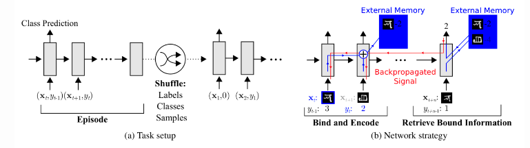
In this way, MANN is motivated to memorize the information of a new dataset, because the memory has to hold the current input until the label is present later, and then retrieve the old information to make a prediction accordingly.

Aside from the training process, a new pure content-based addressing mechanism is utilized to make the model better suitable for meta-learning. The read attention is constructed purely based on the content similarity. First, a key feature vector is produced at the time step by the controller as a function of the input . Similar to the NTM, a read weighting vector of elements is computed as the cosine similarity between the key vector and every memory vector row, normalized by softmax. The read vector is a sum of memory records weighted by such weightings.The addressing mechanism for writing newly received information into memory operates a lot like cache replacement policy. The Least Recently Used Access writed is designed for MANN to better work in the scenario of meta-learning.

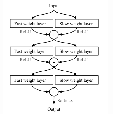
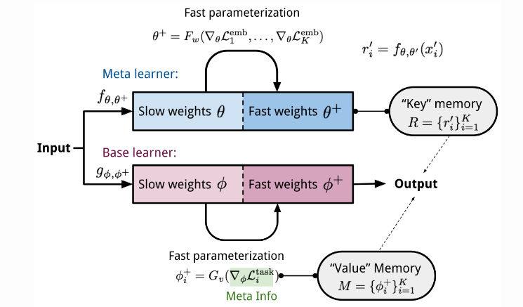
Meta Networks

Meta Networks proposed by Mukhdalai et al. is short of MetaNet, is a meta-learning model with architecture and training process for rapid generalization across tasks. The rapid generalization of MetaNet relies on “fast weights”. Normally, weights in the neural networks are updated by SGD in an objective function and this process is known to be slow. One faster way to learn weights are called fast weights. In MetaNet, loss gradients are used as meta information to populate models that learn fast weights. Slow and fast weights are combined to make predictions in neural networks.

Combining slow and fast weights in a MLP.

Key components of MetaNet are:

• An embedding function , parametrized by , encodes raw inputs into feature vectors. Similar to Siamese Networks, these embeddings are trained to be useful for telling whether two inputs are of the same class.
• A base learner model parameterized by weights , completes the actual learning task. To get fast weights, we need to create two functions and respectively:
• : a LSTM parameterized by for learning fast weights of the embedding function . It takes as input gradients of ’s embedding loss for verification task.
• : a neural network parameterized by learning fast weights for the base learner from its loss gradients. In MetaNet, the learner’s loss gradients are viewed as meta information of the task.

The MetaNet architecture.

Optimization-Based

Deep learning models learn through backpropagation of gradients. However, the gradient-based optimization is neither designed to cope with a small number of training samples, nor to coverage within a small number of optimization steps.

LSTM Meta-Learner

The optimization algorithm can be explicitly modeled. Ravi et al. did so and named it “meta-learner”. The goal of the meta-learner is to efficiently update the learner’s parameters using a small support set so that the learner can adapt to the new tasks quickly. The meta-learner is modeled as a LSTM for two reasons:

• There is a similarity between the gradient based update in backpropagation and the cell-state update in LSTM.
• Knowing a history of gradients benefits the gradient updata.

The update for the learner’s parameters at time step with a learning rate is:. It has the same form as the cell state update in LSTM if we set forget gate , input gate , cell state and new cell state :

While fixing and might not be optimal, both of them can be learnable and adaptable to different datasets. indicates how much to forget the old value of parameters. Whereas, is used as learning rate at time step .

Model setup.

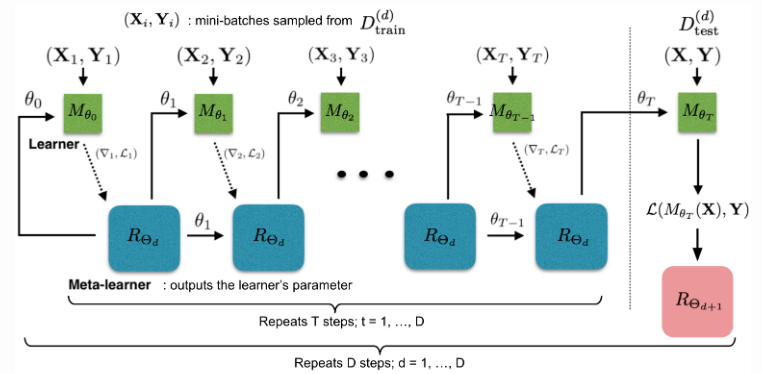
The training process mimics what happens during test. During each training epoch, we first sample a dataset and then sample mini-batches out of train set to update for rounds. The final state of the learner parameter is used to train the meta-learner on the test data.

MAML

MAML is a fairly general optimization algorithm, compatible with any model that learns through gradient descent. The idea is of fine-tuning breaks when transferring to a low data regime, since these approaches were not meant to optimize quickly, and would either overfit to the low data regime or not move far away from their initialization. Meta-learning overcomes this flaw, by taking the point after fine-tuning, and evaluate how well it generalizes to new datapoints for that task (measuring how successful fine-tuning was), and then optimize this objective with regard to the initial set of parameters. We would need to this across all datasets.

Algorithm for MAML.

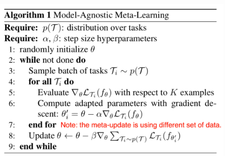
MAML can be viewed as computational graph, with embedded gradient operator. Note that the outer step of MAML assures us that the total loss over all tasks is being optimized, but there is no guarantee for the loss of a given task to be minimized. The meta-optimization step relies on second-order derivatives since, the already has a differentiation step going on. To make computation less expensive, a modified version of MAML omits second derivatives resulting in a simplified and cheaper implementation, known as First-Order MAML.

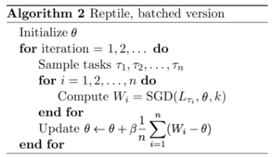
Reptile

Reptile proposed by Nichol et al. is a simple meta-learning optimization algorithm which works by repeatedly:

• Sampling a task
• Training on it by multiple gradient descent steps
• Moving the model weights towards new parameters.

Batched version of Reptile Algorithm.

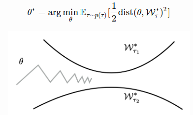
To find a solution that is good across tasks, we would like to find a parameter close to all the optimal manifolds of all tasks.

The Reptile algorithm updates the parameter alternatively to be closer to the optimal manifolds of different tasks.

Probabilistic Interpretation of Optimization-Based Inference

The key idea is to acquire through optimization. Meta-parameters serve as a prior. One form of prior knowledge: initialization for fine-tuning. This initialization can be done as . This is equivalent to using emprical Bayes. This can be approximated to:

where, is the MAP estimate. To compute MAP estimate, we use the following theorem: “Gradient Descent with early stopping is equal to the MAP inference under gaussian prior with mean at initial parameters (this is exactly true in linear case, and approximately true in nonlinear case).” MAML approximates hierrarchical Bayesian inference. Other forms of prior include:

• Gradient descent with explicit gaussian prior:
• Bayesian Linear Regression on learned features
• Closed-form or convex optimization on learned features. Including ridge regression, logistic regression or support vector machines

Some of the challenges in optimization based inference include:

• Selection of architecture for effective inner gradient step: We notice that models that are deep and narrow seem to do well when used with MAML. This can be justified by the fact that a basic architecture + MAML only achieves an accuracy of 63.11% whereas AutoMeta(architecture search) + MAML achieves an accuracy of 74.65% which is a substantial boost.
• Second-order meta-optimization can exhibit instabilities: One of the crude workarounds for this problem includes approximation of the second order gradient to be identity matrix. This idea works well on simple problems, but falls through on more complex problems such as reinforcement learning and imitation learning. Another idea is to automatically learn inner vector learning rate, and tune the outer learning rate (AlphaMAML). Another idea is to optimize only a subset of the parameters in the inner loop. Other ideas include decoupling inner learning rates, and batch norm statistics per step (MAML++) and introducing context variables for increased expressive power.

Bayesian Meta-Learning

parametric approaches use deterministic function (i.e. a point estimate). Since few-shot learning problems may be ambiguous, even with a prior. Hence, using bayesian approach might be better. We would like to generate hypotheses about the underlying function instead. In this method, we use a neural net to produce an intermediate representation which is a Gaussian distribution over . We then train with amortized variational inference (VAE) to obtain variance, etc. of the distribution. This approach is for black-box approach or neural network approach. For optimization based approach, we could model as Gaussian and use the same sort of variational inference as mentioned before, but use the inference network to optimize over . If we do not want to model as Gaussian, we can use Stein Variational Gradient (BMAML) on the last layer of the neural network and use gradient based inference on last layer only. We could also use an ensemble of MAML (EMAML).