Meta Reinforcement Learning

An overview of the talk “Meta Reinforcement Learning DLRL talk” by Chelsea Finn, and “Meta Reinforcement Learning Blog”. In this talk, the author introduces about the concept of Meta Reinforcement Learning. All images and tables in this post are from their talk and blog.

Introduction

The key idea is an pursuit to enable systems to leverage previous experience in order to learn from little data. The goal is to explicitly learn priors from previous experience that lead to efficient downstream tasks. A meta-RL model is trained over a distribution of MDPs, and at test time, it is able to learn to solve a new task quickly. The goal of meta-RL is ambitious, taking one step further towards general algorithms.

Meta-RL Problem Formulation & Examples

The problem formulation is analogous to the meta-learning setting. However, instead, our inputs are the states $s_t$ , and outputs are the actions $a_t$ . Our goal instead to learn the policy $\pi$ that maps states to actions parameterized by $\theta$ such that $a_t = \pi(s_t, \theta)$ . In this scenario, the datasets are analogous to some transitions of the form $\left \{ (s_t, a_t, r_t, s_{t+1}) \right \}$ . Our goal is to learn a policy that maximizes reward. In conclusion, the goal of meta-RL is to leverage previous experience such as $\mathcal{D}_{\mathit{train}}$ (which could be $k$ rollouts from $\pi$ ), and to predict the action for an unknown state $s_t$ such that $a_t = f(\mathcal{D}_{\mathit{train}},s_t;\theta)$ .

Usually the train and test tasks are different but drawn from the same family of problems; i.e., experiments in the papers included multi-armed bandit with different reward probabilities, mazes with different layouts, same robots but with different physical parameters in simulator, and many others. Let’s say we have a distribution of tasks, each formularized as an MDP (Markov Decision Process), $M_i \in \mathcal{M}$ . An MDP is determined by a 4-tuple, $M_i = <\mathcal{S}, \mathcal{A}, \mathcal{P}_i, \mathcal{R}_i>$ . Note that a common state $\mathcal{S}$ and action space $\mathcal{A}$ are used above, so that a (stochastic) policy: $\pi_{\theta}: S \times \mathcal{A} \rightarrow \mathbb{R}_{+}$ would get inputs compatible across different tasks. The test tasks are sampled from the same distribution $\mathcal{M}$ or slightly modified version.

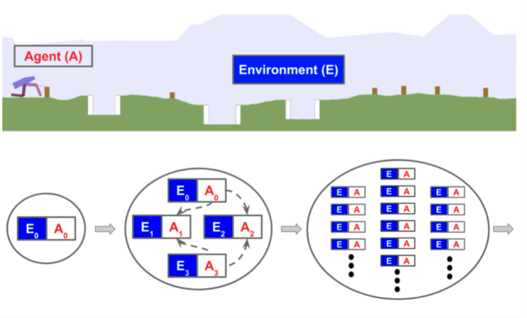
Illustration of meta-RL, containing two optimization loops. The outer loop samples a new environment in every iteration and adjusts parameters that determine the agent’s behavior. In the inner loop, the agent interacts with the environment and optimizes for the maximal reward.

Connection to Contextual Policies

Contextual policy is a policy that is conditioned on some context $\omega$ . For example, $\omega$ could be the position where you want to stack a block in, or maybe the direction that you want to walk in. In many ways, you can view this as a kind of contextual policies or kind of as a special case of these kinds of models. Where, the experience of the data is serving as the context to the policy.

Connections to contextual policies

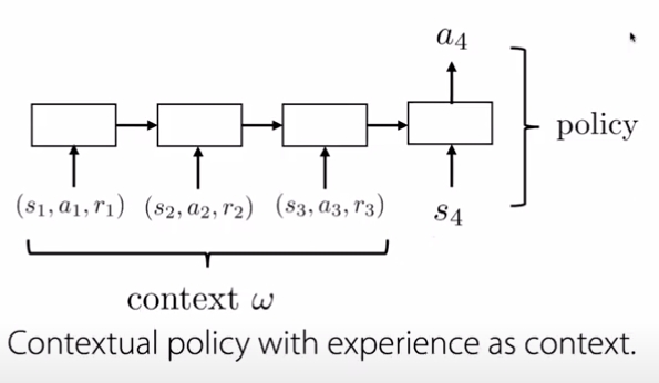
You could view meta-RL as contextual policies with data as context. In meta-RL, the rewards allow you to adapt to any task, even if that task is not a goal reaching task. In that way, these rewards are strict to generalization of goal-based tasks. Furthermore Contextual policies can be viewed as a 0-shot problem, where the goal is to generalize to new goals, rather than adapting to new ones.

Methods

There are two key research directions here, one is the design and optimization of $f$ , and the other is collecting appropriate data (learning to explore) or tasks for prior experience.

Black-Box / Context-Based models

The design of $f$ could be a RNN, an Attention-based network or Temporal Convolutional network. The overall goal is to predict an action for all aggregated states in the inputs.

General working of Reinforcement Learning

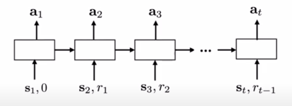
Note that, this takes as input the reward at previous timestep, which is important when we want to adapt to different reward functions. Another difference is that the hidden layers are not maintained across episodes, in order to facilitate easy adaptation to new tasks. These networks are quite general and highly expressive. Furthermore, there is higher flexibility as to how you want to approach the data. A downside to this method is that, the model is quite complex. Learning from complex tasks from scratch is quite difficult, and may require impractical amounts of data in order to adapt properly.

Optimization-Based models

Fine-tuning is the core of optimization-based models. We pre-train the model on a given data, and adapt to a novel dataset. This works quite well in both computer vision setting and natural language processing setting. However, this idea cannot be directly implemented in the few-shot setting. Suppose, you pre-train on ImageNet and then fine-tune on only a few examples, it’s likely to overfit for the small dataset. We need to explicity optimize for the few-shot case, where we perform few adaptations on the new task, and then optimize for those parameters on held out data.

Optimization-based models

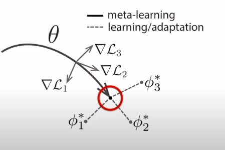
The idea is to reach an optima where fine-tuning to each task is easy, and close, as shown in the highlighted version above. These methods have an inductive bias of SGD built in. They are also model-agnostic, and could be integrated with any architecture. One issue is that RL gradients (policy gradients, or Bellman error) are often not very informative.

Learning to Explore

This section discusses the important problem: “How should we collect $\mathcal{D}_{\mathit{train}}$ ?”

Solution #0:

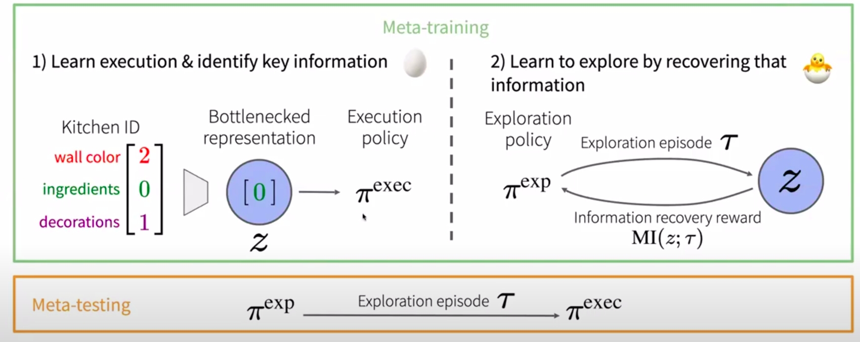
The first solution is to optimize for Exploration & Execution End-to-End w.r.t. reward. The approach is quite simple, and would lead to optimal strategy in principle. However, the downside is that the optimization approach is exceedingly challenging when exploration is difficult. An example of hard exploration meta-rl problem is to learn cooking tasks in previous kitchens. The goal is to quickly learn tasks in a new kitchen. It is quite difficult for the model to understand where all the utensils are, what the environment is, etc. During meta-testing, there are two episodes: one exploration episode to understand where all the equipments are, one for execution.

The reason end-to-end training is hard because we have a chicken and egg problem. We need to do two things, learn how to find ingredients (exploration), and we need to learn how to cook (execution). And if we have a bad exploration policy (cannot find ingredients), and hence, leads to bad execution (cannot learn to cook). Furthermore, if we have a bad execution policy (cannot cook), we would have low reward for any exploration (simply because you cannot cook).

Solution #1:

Another solution is to leverage alternative exploration strategies.

Use posterior sampling: One first learns a distribution over latent task variable $p(z)$ if we have not seen any data, or $q(z|\mathcal{D}_{\mathit{train}})$ if we have seen some data. We also learn the corresponding task policies $\pi(a|s,z)$ for that task. We then sample $z$ from current posterior and sample from policy $\pi(a|s,z)$ . Iteratively reapply the sampling.

Posterior sampling

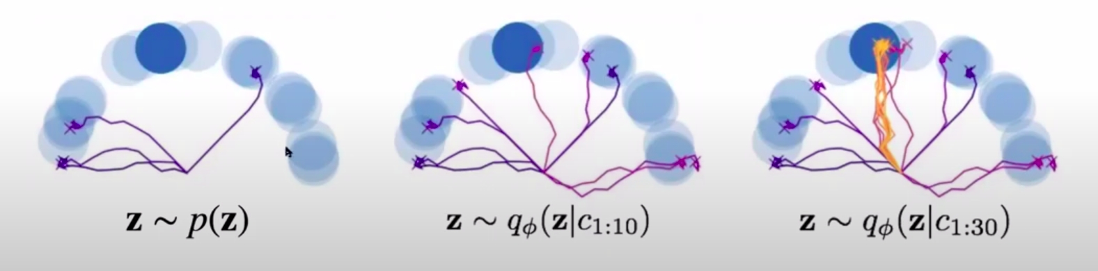
This strategy might not be optimal. Suppose the goal is far away, and there is a sign indicating the path to the sign. The posterior sampling model would not look at the sign, and simply sample goals. The optimal strategy would be to look at the sign.

Another approach is to use intrinsic rewards
Another sample is to predict task dynamics and rewards. In this case, we train the model $f(s',r|s,a,\mathcal{D}_{\mathit{train}})$ . We then collect $\mathcal{D}_{\mathit{train}}$ so that the model is accurate. This may not be optimal where we have a lot of distractors or high dimensional state dynamics.

Many of these methods are easy to optimize, and based on principled strategies. However, these might be suboptimal by arbitrarily large amount in some environments.

Solution #2:

The last solution is to decouple by acquiring representation of task relevant information. This can be theoretically proved to be similar to Solution #0.

Decoupled Reward-free ExplorAtion and Execution in Meta-reinforcement learning(DREAM)

Main Differences from RL

The overall configure of meta-RL is very similar to an ordinary RL algorithm, except that the last reward $r_{t-1}$ and the last action $a_{t-1}$ are also invorporated into the policy observation in addition to the current state $s_{t}$ .

In RL: $\pi_{\theta}(s_t) \rightarrow$ a distribution over $\mathcal{A}$ .
In meta-RL: $\pi_{\theta}(a_{t-1},r_{t-1},s_t)\rightarrow$ a distribution over $\mathcal{A}$ .

The intention of this design is to feed history to the model so that the policy can internalize the dynamics between states, rewards, and actions in the current MDP and adjust its strategy accordingly. Meta-RL generally implement an LSTM policy and the LSTM’s hidden states serve as a memory for tracking characteristics of the trajectories. Becayse the policy is recurrent, there is no need to feed the last state as inputs explicitly.

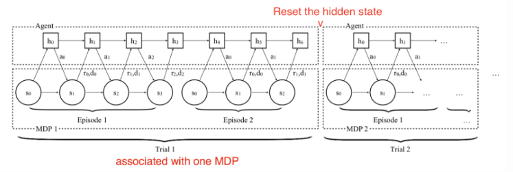
The training procedure works as follows:

Sample a new MDP, $M_i \sim \mathcal{M}$ ;
Reset the hidden state of the model;
Collect multiple trajectories and update the model weights;
Repeat from step 1.

, Illustration of the procedure of the model interacting with a series of MDPs in training time in RL^2 model.

Key Components

There are three key components in Meta-RL:

A model with Memory: A recurrent neural network maintains a hidden state. Thus, it could acquire and memorize the knowledge about the current task by updating the hidden state during rollouts. Without memory, meta-RL would not work.
Meta-learning Algorithm: A meta-learning algorithm refers to how we can update the model weights to optimize for the purpose of solving an unseen task fast at test time. In both Meta-RL and RL^2 papers, the meta-learning algorithm is the ordinary gradient descent update of LSTM with hidden state reset between a switch of MDPs.
A Distribution of MDPs: While the agent is exposed to a variety of environments and tasks during training, it has to learn how to adapt to different MDPs.

The Meta-RL approach involves three pillars: (1) meta-learning architectures, (2) meta-learning algorithms, and (3) automatically generated environments for effective learning.

Meta-Learning Algorithms for Meta-RL

Optimization Model Weights for Meta-Learning

Both MAML and Reptile are methods on updating model parameters in order to achieve good generalization performance on new tasks.

Meta-learning Hyperparameters

The return function in an RL problem, $G_t^{(n)}$ or $G_t^{\lambda}$ , involves a few hyperparameters that are often set heuristically, like the discount factor $\gamma$ and the bootstrapping parameters $\lambda$ . Meta-gradient RL considers them as meta-parameters, $\eta = \{\gamma , \lambda \}$ , that can be tuned and learned online while an agent is interacting with the environment. Therefore, the return becomes a function of $\eta$ and dynamically adapts itself to a specific task over time.

$G_{\eta}^{(n)}(\tau_t) = R_{t+1} + \gamma R_{t+2} + ... + \gamma^{n-1}R_{t+n} + \gamma^n v_{\theta}(s_{t+n})$ \ $G_{\eta}^{\lambda}(\tau_t) = (1-\lambda)\sum_{n=1}^{\infty} \lambda^{n-1}G_{\eta}^{(n)}$

During training, we would like to update the policy parameters with gradients as a function of all the information in hand, $\theta ' = \theta + f(\tau , \theta, \eta)$ , where $\theta$ are the current model weights, $\tau$ is a sequence of trajectories, and $\eta$ are the meta-parameters.

Meanwhile, let’s say we have a meta-objective function $J(\tau, \theta, \eta)$ as a performance measure. The training process follows the principle of online cross-validation, using a sequence of consecutive experiences:

Starting with parameter $\theta$ , the policy $\pi_{\theta}$ is updated on the first batch of samples $\tau$ , resulting in $\theta '$ .
Then we continue running the policy $\pi_{\theta '}$ to collect a new set of experiences $\tau '$ , just following $\tau$ consecutively in time. The performance is measured as $J(\tau ', \theta ', \overline{\eta})$ with a fixed meta-parameter $\overline{\eta}$ .
The gradient of meta-objective $J(\tau ', \theta ', \overline{\eta})$ w.r.t. $\eta$ is used to update $\eta$ .

The meta-gradient RL algorithm simplifies the computation by setting the secondary gradient term to zero, this choice prefers the immediate effect of the meta-parameters $\eta$ on the parameters $\theta$ . Eventually, we get:

$\Delta \eta = \beta \frac{\partial J(\tau ', \theta ', \overline{\eta})}{\partial \theta '} \frac{\partial f(\tau, \theta, \eta)}{\partial \eta}$

Experiments in the paper adopted the meta-objective function same as $\textup{TD}(\lambda)$ algorithm, minimizing the error between the approximated value function $v_{\theta}(s)$ and $\lambda$ -return:

$J(\tau, \theta, \eta) = (G_{\eta}^{\lambda}(\tau)-v_{\theta}(s))^2$ \ $J(\tau ', \theta ', \eta ') = (G_{\overline{\eta}}^{\lambda}(\tau ')-v_{\theta '}(s '))^2$

Meta-learning Loss function

In policy gradient algorithms, the expected total reward is maximized by updating the policy parameters $\theta$ in the direction of estimated gradient:

$g = \mathbb{E}[\sum_{t=0}^{\infty}\Psi_{t}\bigtriangledown _{\theta} \log \pi_{\theta}(a_t|s_t)]$

where the candidates for $\Psi_t$ include the trajectory return $G_t$ , the Q value $Q(s_t, a_t)$ , or the advantage value $A(s_t, a_t)$ . The corresponding surrogate loss function for the policy gradient can be reverse-engineered:

$L_{\textup{PG}} = \mathbb{E}[\sum_{t=0}^{\infty} \Psi_t \log \pi_{\theta}(a_t|s_t)]$

This loss function is a measure over a history of trajectories, ( $s_0, a_0, r_0, ..., s_t, a_t, r_t, ...$ ). Evolved Policy Gradient takes a step further by defining the policy gradient loss function as a temporal convolution (1-D convolution) over the agent’s past experience, $L_{\phi}$ . The parameters $\phi$ of the loss function network are evolved in a way that an agent can achieve higher returns.

Similar to many meta-learning algorithms, EPG has two optimization loops:

In the internal loop, an agent learns to improve its policy $\pi_{\theta}$ .
In the outer loop, the model updates the parameters $\phi$ of the loss function $L_{\phi}$ . Because there is no explicit way to write down a differentiable equation between the return and the loss, EPG turned to Evolutionary Strategies (ES).

A general idea is to train a population of $N$ agents, each of them is trained with the loss function $L_{\phi + \sigma \varepsilon_i}$ parameterized with $\phi$ added with a small gaussian noise $\varepsilon \sim \mathcal{N}(0,\mathbf{I})$ of standard deviation $\sigma$ , During the inner loop’s training, EPG tracks a history of experience and updates the policy parameters according to the loss function $L_{\phi + \sigma \varepsilon_i}$ for each agent:

$\theta_i \leftarrow \theta - \alpha_{\textup{in}} \bigtriangledown_{\theta} L_{\phi + \sigma \varepsilon_i}(\pi_{\theta}, \tau_{t-K,....,t})$

where $\alpha_{\textup{in}}$ is the learning rate of the inner loop and $\tau_{t-K,....,t}$ is a sequence of M transition steps up to the current time step $t$ .

Once the inner loop policy is mature enough, the policy is evaluated by the mean return $\overline{G}_{\phi + \sigma \varepsilon_i}$ over multiple randomly sampled trajectories. Eventually, we are able to estimate the gradient of $\phi$ according to NES numerically. While repeating this process, both parameters $\theta$ and the loss function weights $\phi$ are being updated simultaneously to achieve higher returns.

$\phi \leftarrow \phi + \alpha_{\textup{out}}\frac{1}{\sigma N} \sum_{i=1}^N \varepsilon_i G_{\phi + \sigma\varepsilon_i}$

where $\alpha_{\textup{out}}$ is the learning rate of the outer loop.

In practice, the loss $L_{\phi}$ is bootstrapped with an ordinary policy gradient (such as REINFORCE or PPO) surrogate loss $L_{\textup{PG}}$ , $\widehat{L} = (1-\alpha)L_{\phi} + \alpha L_{\textup{PG}}$ . The weight $\alpha$ is annealing from 1 to 0 gradually during traning. At test time, the loss function parameter $\phi$ stays fixed and the loss value is computed over a history of experience to update the policy parameters $\theta$ .

Meta-learning Exploration Strategies

The exploitation vs exploration dilemma is a critical problem in RL. Common ways to do exploration include $\varepsilon$ -greedy, random noise on actions, or stochastic policy with built-in randomness on the action space.

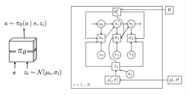
MAESN is an algorithm to learn structured action noise from prior experience for better and more effective exploration. Simply adding random noise on actions cannot capture task-dependent or time-correlated exploration strategies. MAESN changes the policy to condition on a per-task random variable $z_i \sim \mathcal{N}(\mu_i, \sigma_i)$ , for i-th task $M_i$ , so we would have a policy $a \sim \pi_{\theta}(a|s,z_i)$ . The latent variable $z_i$ is sampled once and fixed during one episode. Intuitively, the latent variable determines one type of behavior (or skills) that should be explored more at the beginning of a rollout and the agent would adjust its actions accordingly. Both the policy parameters and latent space are optimized to maximize the total task rewards. In the meantime, the policy learns to make use of the latent variables for exploration.

In addition, the loss function includes the KL divergence between the learned latent variable and a unit Gaussian prior, $D_{\textup{KL}}(\mathcal{N}(\mu_i, \sigma_i)||\mathcal{N}(0,\mathbf{I}))$ . On one hand, it restricts the learned latent space not too far from a common prior. On the other hand, it creates the variational evidence lower bound (ELBO) for the reward function. Interestingly, the paper found that $(\mu_i, \sigma_i)$ for each task are usually close to the prior at convergence.

The policy is conditioned on a latent variable variable $z_i \sim \mathcal{N}(\mu, \sigma)$ that is sampled once every episode. Each task has different hyperparameters for the latent variable distribution, (\mu_i, \sigma_i) and they are optimized in the outer loop.

Episodic Control

A major criticism of RL is on its sample inefficiency. A large number of samples and small learning steps are required for incremental parameter adjustment in RL in order to maximize generalization and avoid catastrophic forgetting of earlier learning.

An episodic memory keeps explicit records of past events and uses these records directly as point of reference for making new decisions (just like metric-based meta-learning).

In MFEC(Model-Free episodic control), the memory is modeled as a big table, storing the action pair $(s,a)$ as key and the corresponding Q-value $Q_{\textup{EC}}(s,a)$ as value. When receiving a new observation $s$ , the Q-value is estimated in an non-parametric way as the average Q-value of top $k$ most similar samples:

$\widehat{Q}_{\textup{EC}} = \left\{\begin{matrix} Q_{EC}(s,a) & &\textup{if} (s,a) \in Q_{\textup{EC}}\\ \frac{1}{k}\sum_{i=1}^k Q(s^{(i)},a)& & \textup{otherwise} \end{matrix}\right.$

where $s^{(i)}, i=1,...,k$ are the top $k$ states with smallest distances to the state $s$ . Then the action yields the highest estimated Q value is selected. Then the memory is updated according to the return received at $s_t$ :

$Q_{\textup{EC}}(s,a) = \left\{\begin{matrix} \max \{Q_{\textup{EC}}(s_t,a_t),G_t\} & & \textup{if} (s,a)\in Q_{\textup{EC}},\\ G_t & & \textup{otherwise} \end{matrix}\right.$

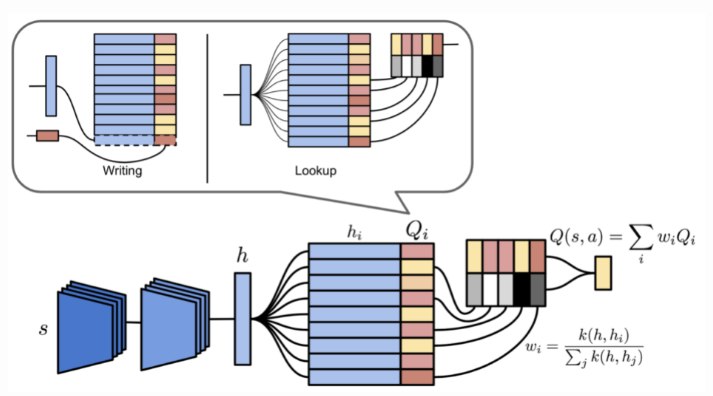
A tabular RL method, MFEC suffers from large memory consumption and a lack of ways to generalize among similar states. The fisrt one can be fixed with an LRU cache. Inspired by metric-based meta-learning, especially Matching Networks, the generalization problem is improved in a follow-up algorithm, NEC (Neural Episodic Control).

The episodic memory in NEC is Differentiable Neural Dictionary (DND), where the key is a convolutional embedding vector of input image pixels and the value stores estimated Q value. Giving an inquiry key, the output is a weighted sum of values of top similar keys, where the weight is a normalized kernel measure between the query key and selected key in the dictionary. This sounds like a hard attention mechanism.

Illustrations of episodic memory module in NEC an two operations on a differentiable neural dictionary.

Further, Episodic LSTM enhances the basic LSTM achitecture with a DND episodic memory, which stores task context embeddings as keys and the LSTM cell states as values. The stored hidden states are retrieved and added directly to the current cell state through the same gating mechanism within LSTM:

Illustrations of episodic LSTM architecture. The additional structure of episodic memory is in bold.

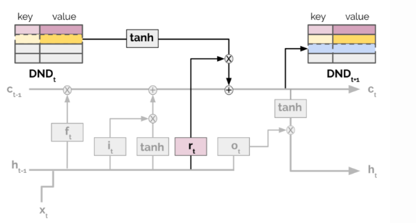
The architecture provides a shortcut to the prior experience through context-based retrieval. Meanwhile, explicitly saving the task-dependent experience in an external memory avoids forgetting. In the paper, all experiments have manually designed context vectors. How to construct an effective and efficient format of task context embeddings for more free-formed tasks would be an interesting topic.

Overall, the capacity of episodic control is limited by the complexity of the environment. It is very rare for an agent to repeatedly visit exactly the same states in a real-world task, so properly encoding the states is critical. The learned embedding space compresses the observational data into a lower dimensional space, and, in the meantime, two states being close in this space are expected to demand similar strategies.

Training Task Acquisition

Among the three key components, how to design a proper distribution of tasks is the less studied and probably the most specific one to meta-RL itself. As described earlier, each task is a MDP: $M_i = <\mathcal{S},\mathcal{A},\mathcal{P}_i, \mathcal{R}_i> \in \mathcal{M}$ . We can build a distribution of MDPs by modifying:

The reward configuration: Among different tasks, the same behavior might get rewarded differently according to $\mathcal{R}_i$ .
Or, the environment: The transition function $\mathcal{P}_i$ can be reshaped by initializing the environment with varying shifts between states.

Task Generation by Domain Randomization

Randomizing parameters in a simulator is an easy way to obtain tasks with modified transition functions.

Evolutionary Algorithm on Environment Generation

Evolutionary algorithm is a gradient-free heuristic-based optimization method, inspired by natural selection. A population of solutions follows a loop of evaluation, selection, reproduction, and mutation. Every good solutions survive and thus get selected.

POET, a framework based on the evolutionary algorithm, attempts to generate tasks while the problems themselves are being solved. The implementation of POET is only specifically designed for a simple 2D bipedal walker environment but points out an interesting direction. It is noteworthy that the everloutionary algorithm has had some compelling applications in Deep Learning.

The 2D bipedal walking environment is evolving: from a simple flat surface to a much more difficult trail with potential gaps, stumps and rough terrains. POET pairs the generation of environmental challenges and optimization of agents together so as to (a) select agents that can resolve current challenges and (b) evolve environments to be solvable. The algorithm maintains a list of environment agent pairs and repeats the following:

Mutation: Generate new environments from currently active environments. Note that here types of mutation operations are created just for bipedal walker and a new environment would demand a new set of configurations.
Optimization: Train paired agents within their respective environments.
Selection: Periodically attempt to transfer current agents from one environment to another. Copy and update the best performing agent for every environment. The intuition is that skills learned in one environment might be helpful for a different environment.

The procedure above is quite similar to PBT, but PBT mutates and evolves hyperparameters instead. To some extent, POET is doing domain randomization, as all gaps, stumps and terrain roughness are controlled by some randomization probability parameters. Different from DR, the agents are not exposed to a fully randomized difficult environment all at once, but instead they are learning gradually with a curriculum configured by the evolutionary algorithm.

An example bipedal walking environment(top) and an overview of POET(bottom).

Learning with Random Rewards

An MDP without a reward function $R$ is known as Controlled Markov Process (CMP). Given a predifined CMP, $<\mathcal{S},\mathcal{A},\mathcal{P}>$ , we can acquire a variety of tasks by generating a collection of reward functions $\mathcal{R}$ that encourage the training of an effective meta-learning policy.

There are two unsupervised approaches for growing the task distribution in the context of CMP. Assuming there is an underlying latent variable $z \sim p(z)$ associated with every task, it parameterizes/determines a reward function: $r_z(s) = \log D(z|s)$ , where a “discriminator” function $D(.)$ is used to extract the latent variables from the state. There are two ways to create this discriminator function:

Sample random weights $\phi_{\textup{rand}}$ of the discriminator, $D_{\phi_{\textup{rand}}}(z|s)$ .
Learn a discriminator function to encourage diversity-driven exploration. This method was introduced in a paper called “DIAYN”.

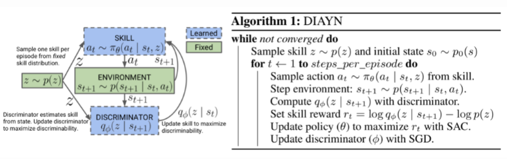
DIAYN (Diversity is all you need), is a framework to encourage a policy to learn useful skills without a reward function. It explicitly models the latent variables $z$ as a skill embedding, and makes the policy conditioned on this latent variable, in addition to state: $\pi_{\theta}(a|s,z)$ . The design of DIAYN is motivated by a few hypotheses:

Skills should be diverse and lead to visitations of different states. This helps maximize the mutual information between states and skills, $I(S;Z)$ .
Skills should be distinguished by states, not actions. This helps minimize the mutual information between actions and skills, conditioned on states $I(A;Z|S)$ .

The objective function to maximize is as follows, where the policy entropy is also added to encourage diversity:

$\mathcal{F}(\theta) = I(S;Z) + H[A|S] - I(A;Z|S)$ \ $= (H(Z)-H(Z|S)) + H[A|S] - (H[A|S]-H[A|S,Z])$ \ $= H[A|S,Z] + {\color{Green} H(Z)-H(Z|S)}$ \ $= H[A|S,Z] + \mathbb{E}_{z\sim p(z), s\sim \rho (s)}[\log p(z|s)] - \mathbb{E}_{z\sim p(z)}[\log p(z)]$ \ $\geq H[A|S,Z] + \mathbb{E}_{z\sim p(z), s\sim \rho (s)}[{\color{Red} \log D_{\phi}(z|s) - \log p(z)}]$

The above equation can infer skills from state $s$ and $p(z)$ is diverse. Furthermore, according to Jensen’s inequality; “pseudo-reward” is represented in red.

Here, $I(.)$ is mutual information and $H[.]$ is entropy measure. We cannot integrate all states to compute $p(z|s)$ , so approximate it with $D_{\phi}(z|s)$ - that is the diversity-driven discriminator function.

Once the discriminator is learned, sampling a new MDP for training is straight-forward: First, we sample a latent variable, $z \sim p(z)$ and construct a reward function $r_z(s) = \log (D(z|s))$ . Pairing the reward function with a predefined CMP creates a new MDP.

DIAYN Algorithm.

Challenges & Latest Developments

Some of the open-ended problems include:

Adapting to entirely new tasks or dataset - Meta-World benchmark as a starting point?
Robustness to out of distribution tasks
Where do the tasks even come from
Need better RL algorithms

Written on October 9, 2021