Reinforcement Learning

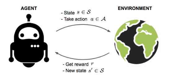
An overview of the topic “A (Long) Peek into Reinforcement Learning”. Say, we have an agent in an unknown environment and this agent can obtain some rewards by interacting with the environment. The agent ought to take actions so as to maximize cumulative rewards. The goal of Reinforcement Learning (RL) is to learn a good strategy for the agent from experimental trials and relatively simple feedback received. With the optimal strategy, the agent is capable to actively adapt to the environment to maximize future rewards.

An agent interacts with the environment, trying to take smart actions to maximize cumulative rewards.

Background

The agent is acting in an environment. How the environment reacts to certain actions is defined by a model which we may or may not know. The agent can stay in one of the many states ( $s \in S$ ) of the environment, and choose to take one of the many actions ( $a \in A$ ) to switch from one state to another. Which state the agent will arrive in is decided by transition probabilities between states ( $P$ ). Once an action is taken, the environment delivers a reward ( $r \in R$ ) as feedback.

The model defines the reward functions and transition probabilities. We may or may not know how the model works and this differentiate two circumstances:

Know the model: planning with perfect information; do model-based RL. When we fully know the environment, we can find the optimal solution by Dynamic Programming.
Do not know the model: learning with incomplete information; do model-free RL or try to learn the model explicitly as part of the algorithm. Most of the following content serves the scenarios when the model is unknown.

The agent’s policy ( $\pi(s)$ ) provides the guidelines on what is the optimal action to take in a certain state with the goal to maximize total rewards. Each state is associated with a value function $V(s)$ predicting the expected amount of future rewards we are able to receive in this state by acting the corresponding policy. In other words, the value function quantifies how good a state is. Both policy and value functions are what we try to learn in reinforcement learning.

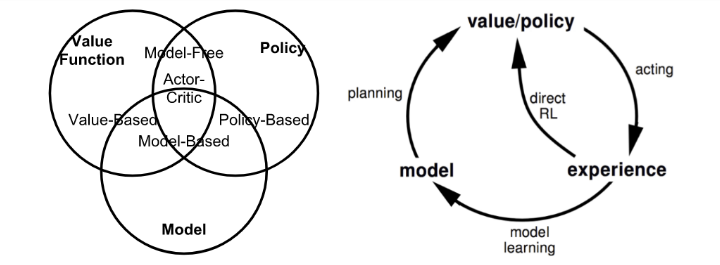
Summary of approaches in RL based on whether we want to model the value, policy, or the environment.

The interaction between the agent and the environment involves a sequence of actions and observed rewards in time, $t = 1,2,...,T$ . During the process, the agent accumulates the knowledge about the environment, learns the optimal policy, and makes decisions on which action to take next so as to efficiently learn the best policy. Let’s label the state, action, and reward at time step $t$ as $S_t$ , $A_t$ , and $R_t$ , respectively. Thus, the interaction sequence is fully described by one episode (also known as “trial” or “trajectory”) and the sequence ends at the terminal state $S_T$ :

$S_1,A_1,R_2,S_2,A_2,....,S_T$

Some important terms in RL algorithms involve:

Model-based: Rely on the model of the environment; either the model is known or the algorithm learns it explicitly.
Model-free: No dependency on the model during learning.
On-policy: Use the deterministic outcomes or samples from the target policy to train the algorithm.
Off-policy: Training on a distribution of transitions or episodes produced by a different behavior policy rather than that produced by the target policy.

Model: Transition and Reward

The model is a descriptor of the environment. With the model, we can learn or infer how the environment would interact with and provide feedback to the agent. The model has two major parts, transition prbability function $P$ , and reward function $R$ .

Suppose, we are in state $s$ , we decide to take action $a$ to arrive in the next state $s'$ and obtain reward $r$ . This is known as one transition step represented by a tuple $(s,a,s',r)$ .

The transition function $P$ records the probability of transitioning from state $s$ to $s'$ after taking action $a$ while obtaining reward $r$ . We use $\mathbb{P}$ as a symbol of probability.

$P(s',r|s,a) = \mathbb{P}[S_{t+1}=s', R_{t+1}=r|S_t=s, A_t=a]$

Thus, the state-transition function can be defined as a function of $P(s',r|s,a)$ :

$P_{ss'}^a = P(s'|s,a) = \sum _{r\in \mathcal{R}} P(s',r|s,a)$

Similarly, the reward function $R$ predicts the next reward triggered by a given action:

$R(s,a) = \mathbb{E}[R_{t+1}|S_t=s,A_t=a] = \sum _{r \in \mathcal{R}} r \sum_{s' \in S} P(s',r|s,a)$

Policy

Policy is defined as the agent’s behavior function $\pi$ , and tells us which action to take in state $s$ . It is a mapping from state $s$ to action $a$ and can either be deterministic or stochastic.

Deterministic: $\pi(s) = a$
Stochastic: $\pi(a|s) = \mathbb{P}_{\pi}[A=a|S=s]$

Value function

Value function measures the goodness of a state, or how rewarding a state or action is by predicting future reward. The future reward is also known as return, and is the total sum of discounted rewards going forward.

$G_t = R_{t+2} + \gamma R_{t+2} + .. = \sum_{k=0}^\infty \gamma ^{k} R_{t+k+1}$

The discounting factor $\gamma \in [0,1]$ penalize the rewards in the future for few reasons:

The future rewards may have higher uncertainty.
The future rewards do not provide immediate benefits.
Discounting provides mathematical convenieve; we can make approximations .
We do not need to worry about the infinite loops in state transition graph.

The state-value of a state $s$ is the expected return if we are in this state at time $t$ , $S_t = s$ :

$V_{\pi}(s) = \mathbb{E}[G_t|S_t=s]$

Similarly, we define the action-value (“Q-value”) of a state-action pair as:

$Q_{\pi}(s,a) = \mathbb{E}_{\pi}[G_t|S_t=s,A_t=a]$

Additionally, since we follow the target policy $\pi$ , we can make use of the probility distribution over possible actions and the Q-values to recover the state-value:

$V_{\pi}(s) = \sum_{a \in \mathcal{A}} Q_{\pi}(s,a)\pi(a|s)$

The difference between action-value and state-value is the action advantage function (“A-value”):

$A_{\pi}(s,a) = Q_{\pi}(s,a) - V_{\pi}(s)$

This can be thought of as the advantage of selecting an action $a$ in a given state $s$ compared to all other actions available to you.

Optimal Value and Policy

The optimal value function produces the maximum return:

$V_{*}(s) = \max_{\pi} V_{\pi}(s), Q_{*}(s,a) = \max_{\pi} Q_{\pi}(s,a)$

The optimal policy achieves optimal value functions:

$\pi_{*} = \arg \max_{\pi} V_{\pi}(s), \pi_{*} = \arg \max_{\pi} Q_{\pi}(s,a)$

Markov Decision Processes

In formal terms, almost all RL problems can be framed as Markov Decision Processses (MDPs). All states in MDP have “Markov” property, referring to the fact that the future only depends on the current state, not the history:

$\mathbb{P}[S_{t+1}|S_t] = \mathbb{P}[S_{t+1}|S_1,...,S_t]$

In other words, the future and the past are conditionally independent given the present, as the current state encapsulates all the statistics we need to decide the future.

The agent-environment interaction in a Markov decision process.

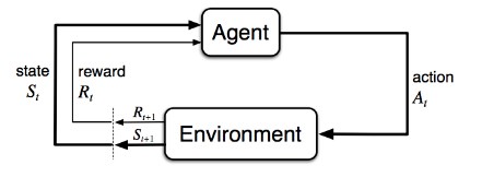
A Markov decision process consists of five elements $\mathcal{M} = < \mathcal{S}, \mathcal{A},\mathcal{P},\mathcal{R},\gamma>$ , where the symbols have the same meanings as discussed in previous sections. Note that, in an unknown environment, we do not have perfect knowledge about $\mathcal{P}$ and $\mathcal{R}$ .

Bellman Equations

Bellman equations refer to the set of equations that decompose the value function into the immediate reward plus the discounted future values.

$V(s) = \mathbb{E}[G_t|S_t=s]$ $= \mathbb{E}[R_{t+1} + \gamma R_{t+2}+\gamma^2 R_{t+3}+...|S_t=s]$ $= \mathbb{E}[R_{t+1} + \gamma (R_{t+2}+\gamma R_{t+3}+...)|S_t=s]$ $= \mathbb{E}[R_{t+1} + \gamma G_{t+1}|S_t=s]$ $= \mathbb{E}[R_{t+1} + \gamma V(S_{t+1})|S_t=s]$

Similarly, for Q-value,

$Q(s,a) = \mathbb{E}[R_{t+1} + \gamma V(S_{t+1})|S_t=s, A_t=a]$ $= \mathbb{E}[R_{t+1} + \gamma \mathbb{E}_{a' \sim \pi}Q(S_{t+1},a')|S_t=s, A_t=a]$

Bellman Expectation Equations

The recursive update process can be further decomposed to be equations built on both state-value functions. As we go further in future action steps, we extend $V$ and $Q$ alternatively by following the policy $\pi$ .

$V_{\pi}(s) = \sum_{a \in \mathcal{A}} \pi(a|s) Q_{\pi}(s,a)$ $Q_{\pi}(s,a) = R(s,a) + \gamma \sum_{s' \in \mathcal{S}} P^a_{ss'} V_{\pi}(s')$ $V_{\pi}(s) = \sum_{a\in \mathcal{A}} \pi(a|s)(R(s,a) + \gamma \sum_{s'\in \mathcal{s}} P^a_{ss'}V_{\pi}(s'))$ $Q_{\pi}(s,a) = R(s,a) + \gamma \sum_{s'\in \mathcal{S}} P^a_{ss'} \sum_{a' \in \mathcal{A}} \pi(a'|s')Q_{\pi}(s',a')$

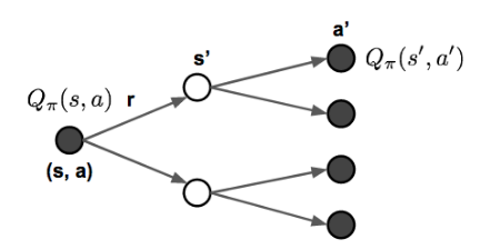
Illustration of how Bellman expectation equations update state-value and action-value functions.

If we are interested in the optimal values rather than computing the expectation following a policy, we could jump right into the maximum returns during the alternative updates without using a policy. If we have complete information of the environment, this turns into a planning problem, solvable by DP. Unfortunately, in most scenarios, we do not know $P^a_{ss'}$ or $R(s,a)$ , so we cannot solve MDPs by directly applying Bellmen equations, but it lays the theoretical foundation for many RL algorithms.

Common Approaches

In this section, we discuss some of the common approaches and classical algorithms used for solving RL problems.

Dynamic Programming

When the model is fully known, following Bellman equations, we can use DP to iteratively evaluate the value functions and improve policy.

Policy Evaluation

Policy evaluation is to compute the state-value $V_{\pi}$ for a given policy $\pi$ :

$V_{t+1}(s) = \sum_{a} \pi(a|s) \sum_{s',r} P(s',r|s,a)(r+\gamma V_t(s'))$

Policy Improvement

Based on the value functions, Policy improvement generates a better policy by acting greedily.

$Q_{\pi}(s,a) = \sum_{s',r} P(s',r|s,a)(r+\gamma V_t(s'))$

Policy iteration

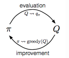
The Generalized Policy Iteration (GPI) algorithm refers to an iterative procedure to improve the policy when combining policy evaluation and improvement.

$\pi_0 \xrightarrow[]{\textup{evaluation}} V_{\pi_0} \xrightarrow[]{\textup{improve}} \pi_1 \xrightarrow[]{\textup{evaluation}} V_{\pi_1} \xrightarrow[]{\textup{improve}} \pi_2 \xrightarrow[]{\textup{evaluation}} ... \xrightarrow[]{\textup{improve}} \pi_{*} \xrightarrow[]{\textup{evaluation}} V_{*}$

In GPI, the value function is approximated repeatedly to be closer to the true value of the current policy, and in meantime, the policy is improved repeatedly to approach optimality. Say, we have a policy $\pi$ and then generate an improved version $\pi '$ by greedily taking actions, $\pi '(s) = \arg \max_{a\in \mathcal{A}} Q_{\pi}(s,a)$ .

Monte-Carlo Methods

Monte-Carlo (MC methods use a simple idea: It learns from episodes of raw experience without modeling the environmental dynamics and computes the observed mean return as an approximation of the expected return. To compute the empirical return $G_t$ , MC methods need to learn from complete episodes: $S_1, A_1, R_2, ..., S_T$ to compute $G_t = \sum_{k=0}^{T-t-1} \gamma^k R_{t+k+1}$ and all episodes must eventually terminate. THe empirical mean return for state $s$ is:

$V(s) = \frac{\sum_{t=1}^T \mathbb{I}[S_t=s]G_t}{\sum_{t=1}^T \mathbb{I}[S_t=s]}$

where, $\mathbb{I}[S_t=s]$ is a binary indicator function. We may count the visit of state $s$ every time so that there could exist multiple visits of one state in one episode, or only count it the first time we encounter a state in one episode. This way of approximation can easily be extended to action-value functions by counting $(s,a)$ pair.

$Q(s,a) = \frac{\sum _{t=1}^T \mathbb{I}[S_t=s, A_t=a]G_t}{\sum _{t=1}^T \mathbb{I}[S_t=s, A_t=a]}$

Illustration of MC approach.

To learn the optimal policy by MC, we iterate it by following a similar idea to GPI.

We improve the policy greedily with respect to the current value function: $\pi(s) = \arg \max_{a\in \mathcal{A}} Q(s,a)$ .
Generate a new episode with the new policy $\pi$
Estimate $Q$ using the new episode: $q_{\pi}(s,a) = \frac{\sum_{t=1}^T (\mathbb{I}[S_t=s, A_t=a] \sum_{k=0}^{T-t-1}\gamma^kR_{t+k+1})}{\sum_{t=1}^T \mathbb{I}[S_t=s, A_t=a] }$

Temporal-Difference Learning

Similar to Monte-Carlo methods, Temporal Difference (TD) learning is model-free and learns from episodes of experience. However, TD learning can learn from incomplete episodes and hence we don’t need to track the episode up to termination.

Bootstrapping

TD learning methods update targets with regard to existing estimates rather than exclusively relying on actual rewards and complete returns as in MC methods. This approach is known as bootstrapping.

Value Estimation

The key idea in TD learning is to update the value function $V(S_t)$ towards an estimated return $R_{t+1}+\gamma V(S_{t+1})$ (known as “TD target”). To what extent we want to update the value function is controlled by the learning rate hyperparameter $\alpha$ :

$V(S_t) \leftarrow (1-\alpha)V(S_t) + \alpha G_t$ \ $V(S_t) \leftarrow V(S_t) + \alpha (G_t - V(S_t))$ \ $V(S_t) \leftarrow V(S_t) + \alpha (R_{t+1} + \gamma V(S_{t+1}) - V(S_t))$

Similarly, for the action-value estimation:

$Q(S_t,A_t) \leftarrow Q(S_t, A_t) + \alpha (R_{t+1} + \gamma Q(S_{t+1}, A_{t+1}) - Q(S_t, A_t))$

SARSA: On-Policy TD control

“SARSA” refers to the procedure of updating Q-value by following a sequence of $..., S_t, A_t, R_{t+1},S_{t+1}, A_{t+1}, ...$ . The idea follows the same route of GPI. A brief explanation of the algorithm is as follows:

Initialize $t=0$ .
Start with $S_0$ and choose action $A_0 = \arg \max_{a \in \mathcal{A}} Q(S_0,a)$ , where $\varepsilon$ -greedy is commonly applied.
At time $t$ , after applying action $A_t$ , we observe reward $R_{t+1}$ and get into the next state $S_{t+1}$ .
Then pict the next action in the same way.
Update the Q-value function:

$Q(S_t,A_t) \leftarrow Q(S_t, A_t) + \alpha (R_{t+1} + \gamma Q(S_{t+1}, A_{t+1}) - Q(S_t, A_t))$

Set $t = t+1$ and repeat from step 3.

In each step of SARSA, we need to choose the next action according to the current policy.

Q-Learning: Off-policy TD control

The development of Q-learning is a big breakout in the early days of Reinforcement Learning. Within one episode, it works as follows:

Initialize $t=0$ .
Start with $S_0$
At time step $t$ , we pick the action according to Q values, $A_t = \arg \max_{a\in \mathcal{A}} Q(S_t, a)$ and $\varepsilon$ -greedy is commonly applied.
After applying action $A_t$ , we observe reward $R_{t+1}$ and get into the next state $S_{t+1}$ .
Update the Q-value function:

$Q(S_t, A_t) \leftarrow Q(S_t, A_t) + \alpha(R_{t+1} + \gamma Q(S_{t+1},A_{t+1}) - Q(S_t, A_t))$

Set $t = t+1$ and repeat from step 3.

The key difference from SARSA is that Q-learning does not follow the current policy to pick the second action $A_{t+1}$ . It estimates $Q^{*}$ out of the best Q values, but which action (denoted as $a^{*}$ ) leads to this maximal Q does not matter. Instead, in the next step Q-learning may not follow $a^{*}$ .

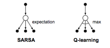
The backup diagrams for Q-learning and SARSA.

Deep Q-Network

Combining TD and MC Learning

In the previous section on value estimation in TD learning, we only trace one step further down the action chain when calculating the TD target. One can easily extend it to take multiple steps to estimate the return.

Let’s label the estimated return followin $n$ steps as $G_t^{(n)}$ , $n = 1,...,\infty$ , then:

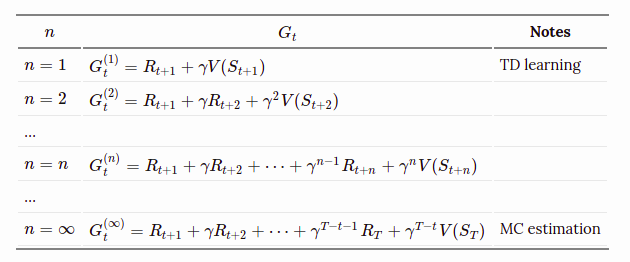
The generalized n-step TD learning still has the same form of value function:

$V(S_t) \leftarrow V(S_t) + \alpha(G_T^{(n)} - V(S_t))$

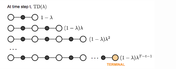
We are free to pick any $n$ in TD learning as we like. Now, the question becomes what is the best $n$ ? Which $G_t^{(n)}$ gives us the best return approximation? A common yet smart solution is to apply a weighted sum of all possible n-step TD targets rather than pick the best $n$ . The weight decay by a factor $\lambda$ with n, $\lambda^{n-1}$ ; the intuition is similar to why we want to discount future rewards when computing tje return: the more future we look into, the less confident we would be. To make all the weight ( $n \rightarrow \infty$ ) sum up to 1, we multiply every weight by ( $1-\lambda$ ).

The weighted sum of many n-step returns is called $\lambda$ -return $G_t^{\lambda} = (1-\lambda)\sum_{n=1}^{\infty} \lambda^{n-1}G_t^{(n)}$ . TD learning that adopts $\lambda$ -return for value updating is labeled as TD( $\lambda$ ). The original version introduced above is equivalent to TD(0).

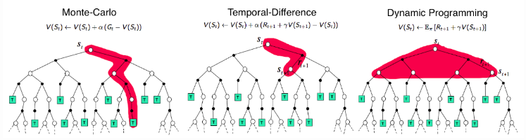
Comparison of backup diagrams of Monte-Carlo, Temporal-Difference learning, and Dynamic Programming for state value functions.

Policy Gradient

All the methods we have introduced above aim to learn the state/action function and then to select actions accordingly. Policy gradient methods instead learn the policy directly with a parameterized function with respect to $\theta$ , $\pi(a|s;\theta)$ . Let’s define the reward function (opposite of loss function) as the expected return and train the algorithm with the goal to maximize the reward function. In discrete space:

$\mathcal{J}(\theta) = V_{\pi_{\theta}}(S_1) = \mathbb{E}_{\pi_{\theta}}[V_1]$

where $S_1$ is the initial starting state.

Or in continuous space:

$\mathcal{J}(\theta) = \sum_{s\in \mathcal{S}}d_{\pi_{\theta}}(s) \sum_{a\in \mathcal{A}}\pi(a|s,\theta)Q_{\pi}(s,a)$

where $d_{\pi_{\theta}}(s)$ is stationary distribution of Markov chain for $\pi_{\theta}$ . Using gradient ascent, we can find the best $\theta$ that produces the highest return. It is natural to expect policy-based methods are more useful in continuous space, because there is an infinite number of actions and/or states to estimate the values for in continuous space and hence value-based approaches are computationally much more expensive.

Policy Gradient Theorem

Computing the gradient numerically can be done perturbing $\theta$ by a small amount $\varepsilon$ in the k-th dimension. It works wven when $J(\theta)$ is not differentiable, but unsurprisingly very slow.

$\frac{\partial \mathcal{J}(\theta)}{\partial \theta_k} \approx \frac{\mathcal{J}(\theta + \varepsilon u_k) - \mathcal{J}(\theta)}{\varepsilon}$

Or analytically,

$\mathcal{J}(\theta) = \mathbb{E}_{\pi_{\theta}}[r] = \sum_{s\in \mathcal{S}}d_{\pi_{\theta}}(s) \sum_{a\in \mathcal{A}} \pi (a|s;\theta)R(s,a)$

Actually we have nice theoretical support for replacing $d(.)$ with $d_{\pi}(.)$ :

$\mathcal{J}(\theta) = \sum_{s\in \mathcal{S}}d_{\pi_{\theta}}(s) \sum_{a\in \mathcal{A}} \pi (a|s;\theta)Q_{\pi}(s,a) \propto \sum_{s\in \mathcal{S}}d(s) \sum_{a\in \mathcal{A}} \pi (a|s;\theta)Q_{\pi}(s,a)$

This result is named “Policy Gradient Theorem” which lays the theoretical foundation for various policy gradient algorithms:

$\bigtriangledown \mathcal{J}(\theta) = \mathbb{E}_{\pi_{\theta}}[\bigtriangledown \ln \pi(a|s;\theta)Q_{\pi}(s,a)]$

Reinforce

REINFORCE, also known as Monte-Carlo policy gradient, relies on $Q_{\pi}(s,a)$ , an estimated return by MC methods using episode samples, to update the policy parameter $\theta$ .

A commonly used variation of REINFORCE is to subtract a baseline value from the return $G_t$ to reduce the variance of gradient estimation while keeping the bias unchanged. For example, a common baseline is state-value, and if applied, we would use $A(s,a)=Q(s,a)-V(s)$ in the gradient ascent update.

Initialize $\theta$ at random.
Generate one episode: $S_1, A_1, R_2, S_2, A_2, ..., S_T$
For :
- Estimate the return $G_t$ since the time step $t$ .
- $\theta \leftarrow \theta + \alpha \gamma^t \bigtriangledown \ln \pi(A_t|S_t, \theta)$ .

Actor-Critic

If the value function is learned in addition to the policy, we would get Actor-Critic algorithm.

Critic: updates value function parameters $w$ and depending on the algorithm it could be action-value $Q(a|s;w)$ or state value $V(s;w)$ .
Actor: updates policy parameters $\theta$ , in the direction suggested by the critic, $\pi(a|s,\theta)$ .
Initialize $s$ , $\theta$ , $w$ at random; sample $a \sim \pi(a|s;\theta)$ .
For :
- Sample reward $r_t \sim R(s,a)$ and next state $s' \sim P(s'|s,a)$ .
- Then sample the next action $a' \sim \pi(s',a';\theta)$ .
- Update policy parameters: $\theta \leftarrow \theta + \alpha+{\theta}Q(s,a;w)\bigtriangledown _{\theta}\ln \pi(a|s;\theta)$ .
- Compute the correction for action-value at time t: $G_{t:t+1} = r_t + \gamma Q(s',a';w) - Q(s,a;w)$ , and use it to update value function parameters: $w \leftarrow w + \alpha_w G_{t:t+1} \bigtriangledown _w Q(s,a;w)$ .
- Update $a \leftarrow a'$ and $s \leftarrow s'$ .

$a_{\theta}$ and $a_{w}$ are two learning rates for policy and value function parameter updates, respectively.

A3C

Asynchronous Advantage Actor Critic, short for A3C is a classic policy gradient method with the special focus on parallel training. In A3C, the critics learn the state-value function, $V(s;w)$ , while multiple actors are trained in parallel and get synced with global parameters from time to time. Hence, A3C is good for parallel training by default.

The loss function for state-value is to minimize the mean squared error, $\mathcal{J}_v (w) = (G_t-V(s;w))^2$ and we use gradient descent to find the optimal $w$ . This state-value function is used as the baseline in the policy gradient update.

Outline of the A3C Algorithm.

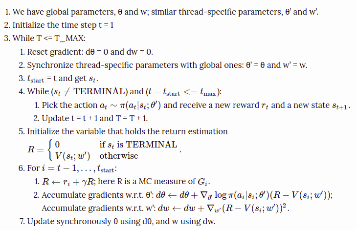
A3C enables the parallelism in multiple agent training. The gradient accumulation step (6.2) can be considered as a reformation of minibatch-based stochastic gradient update: the values of w or θ get corrected by a little bit in the direction of each training thread independently.

Evolution Strategies

Evolution Strategies(ES) is a type of model-agnostic optimization approach. It learns the optimal solution by imitating Darwin’s theory of the evolution of species by natural selection. Two prerequisites for applying ES: (1) our solutions can freely interact with the encironment and see whether they can sove the problem; (2) we are able to compute a fitness score of how good each solution is. We don’t have to know the environment configuration to solve the problem.

Say, we start with a population of random solutions. All of them are capable of interacting with the environment and only candidates with high fitness scores can survive (only the fittest can survive in a competition for limited resources). A new generation is then created by recombining the settings (gene mutation) of high-fitness survivors. This process is repeated until the new solutions are good enough.

Very different from the popular MDP-based approaches as what we have introduced above, ES claims to learn the policy parameter $\theta$ without value approximation. Let’s assume the distribution over the parameter $\theta$ is an isotropic multivariate Gaussian with mean $\mu$ and fixed covariance $\sigma^2 I$ . The gradient of $F(\theta)$ is calculated:

$\bigtriangledown_{\theta} \mathbb{E}_{\theta \sim N(\mu, \sigma ^2)} F(\theta) = \bigtriangledown_{\theta} \int _{\theta} F(\theta)\textup{Pr}(\theta)$
$= \mathbb{E}_{\theta \sim N(\mu, \sigma ^2)} [F(\theta)\frac{\theta - \mu}{\sigma^2}]$

We can rewrite this formula in terms of a “mean” parameter $\theta$ (different from the $\theta$ above; this $\theta$ is the base gene for durther information), $\varepsilon \sim N(0,I)$ and therefore $\theta + \varepsilon \sigma \sim N(\mu, \sigma^2)$ . $\varepsilon$ controls how much Gaussian noises should be added to create mutation:

$\bigtriangledown _{\theta} \mathbb{E}_{\varepsilon \sim N(0,I)} F(\theta + \sigma \varepsilon) = \frac{1}{\sigma} \mathbb{E}_{\varepsilon \sim N(0,I)} [F(\theta + \sigma \varepsilon)\varepsilon]$

ES, as a black-box optimization algorithm, is another approach to RL problems. It has few good characteristics:

ES is fast and easy to train;
ES does not need value function approximation;
ES does not perform gradient back-propagation;
ES is invariant to delayed or long-term rewards;
ES is highly parallelizable with very little data communication.

Known Problems

Exploration-Exploitation Dilemma

When the RL problem faces an unknown environment, this issue is especially key to finding a good solution: without enough exploration, we cannot learn the environment well enough; without enough exploitation, we cannot complete our reward optimization task.

Different RL algorithms balance between exploration and exploitation in different ways. In MC methods, Q-learning or many on-policy algorithms, the exploration is commonly implemented by $\varepsilon$ -greedy; In ES, the exploration is captured by the policy parameter perturbation.

Deadly Triad Issue

We do seek the efficiency and flexibility of TD methods that involve bootstrapping. However, when off-policy, nonlinear function approximation, and bootstrapping are combined to one RL algorithm, the training could be unstable and hard to converge. This issue is known as the deadly triad. Many architectures using deep learning models were proposed to resolve the problem, including DQN to stabilize the training with experience replay and occasionally frozen target network.

Case Study: AlphaGO Zero

The game of Go has been an extremely hard problem in the field of AI. AlphaGo and AlphaGo Zero are two programs developed by a team at DeepMind. Both involve deep CNN and Monte Carlo Tree Search (MCTS), and both have been approved to achieve the level of professional human Go players. Different from AlphaGo that relied on supervised learning from expert human moves, AlphaGo Zero used only reinforcement learning and self-play without human knowledge beyond basic rules.

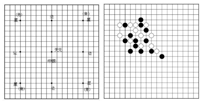
The board of Go. Two players play black and white stones alternatively on the vacant intersections of a board with 19 x 19 lines. A group of stones must have at least one open point (an intersection, called a “liberty”) to remain on the board and must have at least two or more enclosed liberties (called “eyes”) to stay “alive”. No stone shall repeat a previous position.

The main component is a deep CNN over the game board configuration (precisely, a ResNet with batch normalization and ReLU). This network outputs two values:

$(p,v) = f_{\theta}(s)$

$s$ : the game board configuration, 19 x 19 x 17 stacked feature plans; 17 features for each position, 8 past configurations for the current player + 8 past configurations for the opponent + 1 feature indication the color (1=black, 0=white). We need to code the color specifically because the network is playing with itself and the colors of current players and opponents are switching between steps.
$p$ : the probability of selecting a move over 19^2 _1 candidates.
$v$ : the winning probability given the current setting.

AlphaGo Zero is trained by self-play while MCTS improves the output policy further in every step.

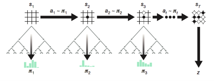
During self-play, MCTS further improves the action probability distribution $\pi \sim p(.)$ and then the action $a_t$ is sampled from this improved policy. The reward $z_t$ is a binary value indicating whether the current player eventually wins the game. Each move generates an episode tuple $(s_t, \pi_t, z_t)$ and it is saved into the replay memory.

The network is trained with the samples in the replay memory to minimize the loss:

$\mathcal{L} = (z-v)^2 - \pi^T \log p + c||\theta||^2$

where $c$ is a hyperparameter controlling the intensity of L2 penalty to avoid overfitting.

AlphaGo Zero simplified AlphaGo by removing supervised learning and merging seperated policy and value networks into one.

Written on October 13, 2021