An overview of the paper “Semi-supervised classification with graph convolutional networks”. The author presents a scalable approach for semi-supervised learning on graph structured data that is based on an efficient variant of CNN which operate directly on graphs. All images and tables in this post are from their paper.

Introduction

Here, the authors consider a problem of classifying nodes in a graph, where labels are only available for a small subset of nodes. This problem can be framed as graph-based semi-supervised learning, where label information is smoothed over the graph via same form of explicit graph-based regularization by using a graph laplacian regularization term in the loss function where:

Here denotes the supervised loss w.r.t. the labeled part of the graph, can be a neural network like differentiable function, is a weighing factor and is a matrix of node features. denotes the unnormalized graph Laplacian of an undirected graph. The above equation relies on the assumption that connected nodes in the graph are likely to share the same label. This assumption, however, might restrict model capacity, as graph edges need not necessarily encode node similarity, but could contain additional information.

Fast approximate convolutions on graphs

Here, we consider a multi-layer Graph Covolutional Network with the following layer-wise propagation rule:

Here, is the adjacency matrix of the undirected graph with added self-connections. is the degree matrix of . A is the adjacency matrix + self loops. This is done so that each node includes its own features at its next representaion. D is the degree matrix of A. Degree matrix is used to normalize nodes with high degrees. denotes the activations of the last layer such that

Spectral Graph convolutions

Here, we consider spectral convolutions on graphs defines as the multiplation of a signal (a scalar for every node) with a filter parametrized by , i.e.:

We can understand as a function of the eigenvalues of the normalized graph Laplacian matrix , with a diagonal matrix of its eigenvalues and is the graph fourier transform of . However, computing the equation is computationally expensive. To circumvent this problem, it was suggested that can be approximated by a truncated expansion in terms of Chebyshev polynomials upto an order of . This approximation only depends only on nodes that are at maximum steps away from the central node.

Layer wise linear Model

A neural network model based on graph colvolutions can therefore be built by stacking multiple convolutional layers of the form described above, each layer followed by a point-wise non-linearity. The idea is that we can recover a rich class of convolutional filter functions by stacking such layers. Intutively, such networks can alleviate the problem of overfitting on local neighborhood structures for graphs with very wide node degree distributions.

In this linear formulation, we only consider immediate neighbors of the node. Successive application of such filters of this form then effectively convolve the order neigborhood of a node, where is the number of successive filterning operations or convolutional layers in a neural network model. To cut down on the number of parameters, we use such that above equation is approximated to:

However, the term now has eigenvalues in the range [0,2]. Repeated application of this operator can therefore lead to numerical instabilities and exploding/vanishing gradiesnt when used in a deep learning model. To alleviate this problem, they introduced the renormalization trick, of using , whose components have been discussed earlier. We finally obtain

which is intuitively similar to computing and propagating these outputs across all nodes using the adjacency matrix.

Graph Convolutional Network

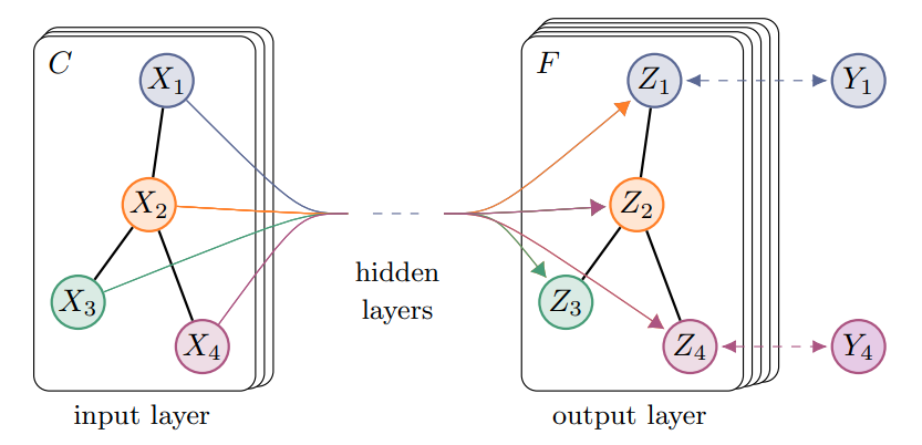
Now, all that’s left is to define a loss function and update using backpropagation and gradient descent.

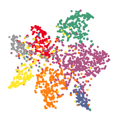
Hidden Layer Activations using TSNE