The Multi-Armed Bandit Problem and Its Solutions

An overview of the topic “The Multi-Armed Bandit Problem and Its Solutions”.

The exploration vs exploitation dilemma exists in many aspects of our life. Say, your favorite restaurant is right around the corner. If you go there every day, you would be confident of what you will get, but miss the chances of discovering an even better option. If you try new places all the time, very likely you are gonna have to eat unpleasant food from time to time.

If we have learned all the information about the environment, we are able to find the best strategy by even just simulating brute-force, let alone many other smart approaches. The dilemma comes from the incomplete information: we need to gather enough information to make best overall decisions while keeping the risk under control. With exploitation, we take advantage of the best option we know. With exploration, we take some risk to collect information about unknown options. The best long-term strategy may involve short-term sacrifices. For example, one exploration trial could be a total failure, but it warns us of not taking that action too often in the future.

Background

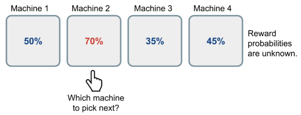
The multi-armed bandit problem is a clssic problem that demonstrates the exploration vs exploitation dilemma well. Imagine you are in a casino facing multiple slot machines and each is configured with an unknown probability of how likely you can get a reward. The question is: What is the best strategy to achieve the highest long-term rewards?

In the blog, the author only covered the case of finite number of trials, and mentioned that this scenario offers a new type of exploration problem. For instance, if the number of trials is smaller than the number of slot machines, we cannot even try every machine to estimate the reward probability and hence we have to behave smartly w.r.t. a limited set of knowledge and resources (i.e. time).

An illustration of how a Bernoulli multi-armed bandit works. The reward probabilities are unknown to the player.

A naive approach can be to continue playing on the machine for many rounds so as to eventually estimate the “true” reward probability. However, this is quite wasteful and does not guarantee the best long-term rewards regardless.

Definitions

A Bernoulli multi-armed bandit can be described as a typle of $<\mathcal{A},\mathcal{R}>$ , where:

We have $K$ machines with reward probabilities, $\{\theta_1, ..., \theta_K\}$ .
At each time step $t$ , we take an action $a$ on one slot machine and receive a reward $r$ .
$\mathcal{A}$ is a set of actions, each referring to the interaction with one slot machine. The value of action $a$ is the expected reward, $Q(a) = \mathbb{E}[r|a] = \theta$ . If action $a_t$ at the time step $t$ is on the i-th machine, then $Q(a_t)=\theta_i$ .
$\mathcal{R}$ is a reward function. In case of Bernoulli bandit, we observe reward $r$ in a stochastic fashion. At time step $t$ , $r_t = \mathcal{R}(a_t)$ may return reward 1 with a probability $Q(a_t)$ or 0 otherwise.

It is a simplified version of Markov decision, as there is no state $\mathcal{S}$ . The goal is to maximize the cumulative reward $\sum_{t=1}^T r_t$ . If we know the optimal action with the best reward, then the goal is same as to minimize the potential regret or loss by not picking the optimal action. The optimal reward probability $\theta^{*}$ of the optimal action $a^{*}$ is:

$\theta^{*} = Q(a^*) = \max_{a\in \mathcal{A}} Q(a) = \max_{1\leq i \leq K} \theta_i$

Our loss function is the total regret we might have by not selecting the optimal selecting the optimal action up to the time step $T$ :

$\mathcal{L}_T = \mathbb{E} [\sum_{t=1}^T (\theta^* - Q(a_t))]$

Based on how we do exploration, there are several ways to solve the multi-armed bandit problem:

No exploration: the most naive approach and a bad one.
Exploration at random
Exploration smartly with a preference to uncertainty.

$\varepsilon$ -Greedy Algorithm

The $\varepsilon$ -greedy algorithm takes the best action most of the time, but does random exploration occasionally. The action value estimated according to the past experience by averaging the rewards associated with the target action $a$ that we have observed so far:

$\widehat{Q}_t(a) = \frac{1}{N_t(a)} \sum_{\tau=1}^t r_{\tau}\mathbb{I}[a_{\tau}=a]$

where $\mathbb{I}$ is a binary indicator function and $N_t(a)$ is how many times the action $a$ has been selected so far, $N_t(a) = \sum_{\tau=1}^t \mathbb{I}[a_{\tau} = a]$ .

According to the $\varepsilon$ -greedy algorithm, with a small probability $\varepsilon$ we take a random action, but otherwise (which should be most of the time), we pick the best action that we have learnt so far.

Upper Confidence Bounds

Random exploration gives us an opportunity to try out options that we have not known much about. However, due to the randomness, it is possible we end up exploring a bad action which we have confirmed in the past (bad luck!). To avoid such inefficient exploration, one approach is to decrease the parameter ε in time and the other is to be optimistic about options with high uncertainty and thus to prefer actions for which we haven’t had a confident value estimation yet. Or in other words, we favor exploration of actions with a strong potential to have a optimal value.

The Upper Confidence Bounds (UCB) algorithm measures this potential by an upper confidence bound of the reward value, $\widehat{U}_t(a)$ , so that the true value is below with bound $Q(a) \leq \widehat{Q}_t(a) + \widehat{U}_t(a)$ with high probability. The upper bound $\widehat{U}_t(a)$ is a function of $N_t(a)$ ; a larger number of trials $N_t(a)$ should give us a smaller bound $\widehat{U}_t(a)$ .

In UCB algorithm, we always select the greediest action to maximize the upper confidence bound:

$a_t^{\textup{UCB}} = \arg \max_{a\in \mathcal{A}} \widehat{Q}_t(a) + \widehat{U}_t(a)$

Hoeffding’s Inequality

If we do not want to assign any prior knowledge on how the distribution looks like, we can get help from “Hoeffding’s Inequality” - a theorem applicable to any bounded distribution.

Let $X_1, ..., X_t$ be the i.i.d. random random variables and they are all bounded by the interval $[0,1]$ . The sample mean is $\overline{X}_t = \frac{1}{t} \sum_{\tau=1}^t X_{\tau}$ . Then for $u > 0$ , we have:

$\mathbb{P}[\mathbb{E}[X] > \overline{X}_t + u] \leq e^{-2tu^2}$

Given one target action $a$ , let us consider:

$r_t(a)$ as the random variables,
$Q(a)$ as the true mean,
$\widehat{Q}_t(a)$ as the sample mean,
And $u$ as the upper confidence bound, $u = U_t(a)$

Then we have, $\mathbb{P}[Q(a)>\widehat{Q}_t(a)+U_t(a)] \leq e^{-2tU_t(a)^2}$ .

We want to pick a bound so that with high chances the true mean is below the sample mean + the upper confidence bound. Thus, $e^{-2tU_t(a)^2}$ should be a small probability. Thus, we set:

$U_t(a) = \sqrt{\frac{-\log p}{2N_t(a)}}$

UCB1

One heuristic is to reduce the threshold $p$ in time, as we want to make more confident bound estimation with more rewards observed. Setting $p = t^{-4}$ , we get UCB1 algorithm:

$U_t(a) = \sqrt{\frac{2log t}{N_t(a)}}$

and,

$a_t^{UCB1} = \arg \max_{a\in \mathcal{A}} Q(a) + \sqrt{\frac{2log t}{N_t(a)}}$

Bayesian UCB

In UCB or UCB1 algorithm, we do not make any prior on the reward distribution and therefore we have to rely on the Hoeffding’s Inequality for a very generalized estimation. If we are able to know the distribution upfront, we would be able to make a better bound estimation.

For instance, if we expect the mean reward of every slot machine to be a Gaussian, we can set the upper bound as 95\% confidence interval by setting $\widehat{U}_t(a)$ to be twice the standard deviation.

Thompson Sampling

At each time step, we want to select action $a$ according to the probability that $a$ is optimal:

$\pi(a|h_t) = \mathbb{P}[Q(a)>Q(a'), \forall a' \neq a |h_t]$ $= \mathbb{E}_{\mathcal{R}|h_t}[\mathbb{I}(a=\arg \max_{a\in \mathcal{A}}Q(a))]$

where $\pi(a|h_t)$ is the probability of taking action $a$ given history $h_t$ .

For the Bernoulli bandit, it is natural to assume that $Q(a)$ follows a Beta distribution, as $Q(a)$ is essentially the success probability $\theta$ in Bernoulli distribution. The value of Beta( $\alpha, \beta$ ) is within the interval $[0,1]$ ; $\alpha$ and $\beta$ correspond to the counts when we succeeded or failed to get a reward respectively.

Initially, we set the Beta parameters based on some prior knowledge or belief. For instance,

$\alpha=1$ and $\beta=1$ ; we expect the reward probability to be around 50\% but are not very confident.
$\alpha=1000$ and $\beta=9000$ ; we strongly believe that the reward probability is 10\%.

At each time $t$ , we sample an expected reward, $\widetilde{Q}(a)$ from the prior distribution $\textup{Beta}(\alpha_i, \beta_i)$ for every action. The best action is selected among samplers. After the true reward is observed, we can update the Beta distribution accordingly, which is essentially doing Bayesian inference to compute posterior with the known prior and the likelihood of getting the sampled data.

$\alpha_i \leftarrow \alpha_i + r_t\mathbb{I}[a_t^{\textup{TS}}=a_i]$ \ $\beta_i \leftarrow \beta_i + (1-r_t)\mathbb{I}[a_t^{\textup{TS}}=a_i]$

Thompson sampling implements the idea of probability matching. Because its reward estimations $\widetilde{Q}$ are sampled from posterior distributions, each of these probabilities is equivalent to the probability that the corresponding action is optimal, conditioned on observed history.

Conclusion

We need exploration because information is valuable. In terms of the exploration strategies, we cannot do exploration at all, focusing on the short-term returns. Or we occasionally explore at random. Or even further, we explore and we are picky about which options to explore — actions with higher uncertainty are favored because they can provide higher information gain.

Summary of algorithms discussed.

Written on October 14, 2021